import pandas as pd
import numpy as np
import matplotlib.pyplot as plt
import seaborn as sns1 Introduction
The analysis is done on Cyclist Trip Data obtained from Coursera Google Data Analytics course as part of Cap Stone Project.
The data contains month wise travel usage of bikes from the year of 2015-2023. We will be concentrating on data gathered in between July-2022 to June-2023 which will cover an entire year.
Let’s load the required packages first
- Loading the required packages i.e.,
pandas,numpy,matplotlib, andseaborn.
2 Loading and Formatting Data
- Let’s look at the structure of the data in one of the downloaded
.csvfiles.
trp_jul_22 = pd.read_csv("F:/Data_Sci/Cap_Stone_Project/Cyclist_trip_data/202207-divvy-tripdata/202207-divvy-tripdata.csv")

trp_jul_22.info()
<class 'pandas.core.frame.DataFrame'>
RangeIndex: 823488 entries, 0 to 823487
Data columns (total 13 columns):
# Column Non-Null Count Dtype
--- ------ -------------- -----
0 ride_id 823488 non-null object
1 rideable_type 823488 non-null object
2 started_at 823488 non-null object
3 ended_at 823488 non-null object
4 start_station_name 711457 non-null object
5 start_station_id 711457 non-null object
6 end_station_name 702537 non-null object
7 end_station_id 702537 non-null object
8 start_lat 823488 non-null float64
9 start_lng 823488 non-null float64
10 end_lat 822541 non-null float64
11 end_lng 822541 non-null float64
12 member_casual 823488 non-null object
dtypes: float64(4), object(9)
memory usage: 81.7+ MB- Let’s look at the columns and try to understand what they represent
ride_idis the unique identification token generated for each ride that was initiated.rideable_typeindicates the type of bike used for the ride.started_atandended_atgive us the time when the ride began and the ride ended respectively.start_station_nameandend_station_namegive us the names of stations where ride began and ended respectively.start_station_idandend_station_idare unique ID’s given to stations.start_latandstart_lngrepresent co-ordinates where the ride began.end_latandend_lngrepresent co-ordinates where the ride stopped.member_casualidentifies if the rider is a member or casual rider of the bike.
- Lets load data of remaining 11 months.
trp_aug_22 = pd.read_csv("F:/Data_Sci/Cap_Stone_Project/Cyclist_trip_data/202208-divvy-tripdata/202208-divvy-tripdata.csv")
trp_sep_22 = pd.read_csv("F:/Data_Sci/Cap_Stone_Project/Cyclist_trip_data/202209-divvy-tripdata/202209-divvy-publictripdata.csv")
trp_oct_22 = pd.read_csv("F:/Data_Sci/Cap_Stone_Project/Cyclist_trip_data/202210-divvy-tripdata/202210-divvy-tripdata_raw.csv")
trp_nov_22 = pd.read_csv("F:/Data_Sci/Cap_Stone_Project/Cyclist_trip_data/202211-divvy-tripdata/202211-divvy-tripdata.csv")
trp_dec_22 = pd.read_csv("F:/Data_Sci/Cap_Stone_Project/Cyclist_trip_data/202212-divvy-tripdata/202212-divvy-tripdata.csv")
trp_jan_23 = pd.read_csv("F:/Data_Sci/Cap_Stone_Project/Cyclist_trip_data/202301-divvy-tripdata/202301-divvy-tripdata.csv")
trp_feb_23 = pd.read_csv("F:/Data_Sci/Cap_Stone_Project/Cyclist_trip_data/202302-divvy-tripdata/202302-divvy-tripdata.csv")
trp_mar_23 = pd.read_csv("F:/Data_Sci/Cap_Stone_Project/Cyclist_trip_data/202303-divvy-tripdata/202303-divvy-tripdata.csv")
trp_apr_23 = pd.read_csv("F:/Data_Sci/Cap_Stone_Project/Cyclist_trip_data/202304-divvy-tripdata/202304-divvy-tripdata.csv")
trp_may_23 = pd.read_csv("F:/Data_Sci/Cap_Stone_Project/Cyclist_trip_data/202305-divvy-tripdata/202305-divvy-tripdata.csv")
trp_jun_23 = pd.read_csv("F:/Data_Sci/Cap_Stone_Project/Cyclist_trip_data/202306-divvy-tripdata/202306-divvy-tripdata.csv")
As structure of .csv’s is same across the all the files lets combine all the .csv files into a single data frame which contains data of all 12 months.
- Combining all the monthly data to one previous year data(
df_1year).
df_1year_raw = pd.concat([trp_jul_22, trp_aug_22, trp_sep_22, trp_oct_22, trp_nov_22,
                      trp_dec_22, trp_jan_23, trp_feb_23, trp_mar_23,
                      trp_apr_23, trp_may_23, trp_jun_23], ignore_index=True)

df_1year_raw.info()
<class 'pandas.core.frame.DataFrame'>
RangeIndex: 5779444 entries, 0 to 5779443
Data columns (total 13 columns):
# Column Dtype
--- ------ -----
0 ride_id object
1 rideable_type object
2 started_at object
3 ended_at object
4 start_station_name object
5 start_station_id object
6 end_station_name object
7 end_station_id object
8 start_lat float64
9 start_lng float64
10 end_lat float64
11 end_lng float64
12 member_casual object
dtypes: float64(4), object(9)
memory usage: 573.2+ MBdf_1yeardata frame contains data from the month of July-2022 to June-2023.
3 Cleaning the Data
- Checking and counting “NA” in each column of the data frame. Data is much better without “NA” as they can cause problems while aggregating data and calculating averages and sums. We can use
mapfunction to perform a function to all of the columns.
df_1year = df_1year_raw.copy()

df_1year.isna().sum()
ride_id 0
rideable_type 0
started_at 0
ended_at 0
start_station_name 857860
start_station_id 857992
end_station_name 915655
end_station_id 915796
start_lat 0
start_lng 0
end_lat 5795
end_lng 5795
member_casual 0
dtype: int64As NA’s are not present in the times columns i.e,
started_atandended_atwe don’t need to worry ourselves aboutNAduring aggregation and manipulation of data but it is a good practice to do so.Finding the length or duration of the rides by making a new column
ride_lengthin minutes and making sure that theride_lengthis not negative by usingif_elsefunction. Eliminating stations where station names and longitude and latitude co-ordinates are not present.
# Converting 'started_at' and 'ended_at' to datetime format
df_1year = df_1year.astype({'started_at': 'datetime64[ns]', 'ended_at': 'datetime64[ns]'})

# Calculating ride length in minutes
df_1year['ride_length'] = (df_1year['ended_at'] - df_1year['started_at']).dt.total_seconds() / 60

# Replacing negative ride lengths with NaN
df_1year['ride_length'] = df_1year['ride_length'].apply(lambda x:0 if x < 0 else x)

# Dropping rows with NaN values in 'ride_length', 'start_station_name',
#  'end_station_name', 'start_lat', 'start_lng', 'end_lat', 'end_lng'

df_1year = ( df_1year[
                    (df_1year['ride_length'] > 0) &
                    (df_1year['start_station_name'].notna()) &
                    (df_1year['end_station_name'].notna()) &
                    (df_1year['start_lat'].notna()) &
                    (df_1year['start_lng'].notna()) &
                    (df_1year['end_lat'].notna()) &
                    (df_1year['end_lng'].notna())
                    ].sort_values('ride_length', ascending=False)
                    )

df_1year.info()
<class 'pandas.core.frame.DataFrame'>
Index: 4408996 entries, 717461 to 4375674
Data columns (total 14 columns):
# Column Dtype
--- ------ -----
0 ride_id object
1 rideable_type object
2 started_at datetime64[ns]
3 ended_at datetime64[ns]
4 start_station_name object
5 start_station_id object
6 end_station_name object
7 end_station_id object
8 start_lat float64
9 start_lng float64
10 end_lat float64
11 end_lng float64
12 member_casual object
13 ride_length float64
dtypes: datetime64[ns](2), float64(5), object(7)
memory usage: 504.6+ MB4 Analysis of Data
Aggregating data by Rider type and Bike type.
- Aggregating data to see “Average minutes per ride” grouped by “bike type” and “rider type” after removing rides less than 2 minutes (As rides less than 2 minutes tend to have the same start and stop stations).
df_1year_agg = (df_1year[df_1year['ride_length'] >= 2]
                     .groupby(['rideable_type', 'member_casual'])
                     .agg(avg_ride_length=('ride_length', 'mean'),
                          total_rides=('ride_length', 'count'),
                          max_ride_length=('ride_length', 'max'))
                     .round(2)
                     .sort_values(by='avg_ride_length', ascending=False)
                     .reset_index()
                     )

df_1year_agg| rideable_type | member_casual | avg_ride_length | total_rides | max_ride_length | |
|---|---|---|---|---|---|
| 0 | docked_bike | casual | 50.44 | 136794 | 32035.45 |
| 1 | classic_bike | casual | 24.80 | 781530 | 1497.75 |
| 2 | electric_bike | casual | 16.03 | 709649 | 479.98 |
| 3 | classic_bike | member | 13.49 | 1630991 | 1497.87 |
| 4 | electric_bike | member | 11.14 | 984688 | 480.00 |
We can clearly notice in Table 1 that member riders have more number of rides with both classic and electric bikes while the average ride length is higher with casual riders.
- Calculating and visualizing Average ride length by “Rider type”.
avg_ride_by_rideable_type = (
    df_1year.rename(columns={'rideable_type': 'Bike Type', 'member_casual': 'Rider Type'})
    .groupby(['Bike Type', 'Rider Type'])
    .agg(
        avg_ride_by_rideable_type=('ride_length', 'mean'),
        total_rides=('ride_length', 'count')
    )
    .reset_index()
)

sns.set(rc={'figure.figsize':(10, 6)})
sns.barplot(data=avg_ride_by_rideable_type,
            x='Rider Type', y='avg_ride_by_rideable_type', hue='Bike Type')
plt.title('Average Ride Length by Rider Type and Bike Type')
plt.xlabel('Rider Type')
plt.ylabel('Average Ride Length (minutes)')
plt.legend(title='Bike Type')
plt.xticks(rotation=45)
plt.tight_layout(rect=[0, 0, 1, 0.96])
plt.show()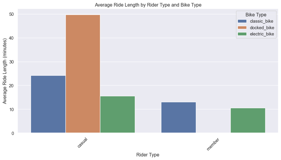
The above Figure 1 clearly shows that members average ride lengths between bike types doesn’t differ much for member riders but differs with casual riders upto 8 minutes.
Note
Further down in the analysis “docked_bike” type is dropped as no proper documentation is available in the course.
4.1 Analysing data by Time of the year and Ride Length
Ride Patterns Across the Weeks and Months of the Year
- Calculating and visualizing ride patterns in a week for number of rides.
# Define the order for rideable_type
rideable_order = ["classic_bike", "electric_bike", "docked_bike"]

# Filter out 'docked_bike'
df_1year_filtered = df_1year[df_1year['rideable_type'] != 'docked_bike'].copy()

# Extracting month and weekday names

df_1year_filtered['month'] = df_1year_filtered['started_at'].dt.month_name()
df_1year_filtered['weekday'] = df_1year_filtered['started_at'].dt.day_name()

# Set categorical order for rideable_type, member_casual, and month

df_1year_filtered['rideable_type'] = pd.Categorical(df_1year_filtered['rideable_type'], categories=rideable_order, ordered=True)

# Set categorical order for member_casual to control legend order
member_order = ['member', 'casual']
df_1year_filtered['member_casual'] = pd.Categorical(df_1year_filtered['member_casual'], categories=member_order, ordered=True)

month_order = ['July', 'August', 'September', 'October', 'November', 'December',
             'January', 'February', 'March', 'April', 'May', 'June']

weekday_order = ['Monday', 'Tuesday', 'Wednesday', 'Thursday', 'Friday', 'Saturday', 'Sunday']

df_1year_filtered['month'] = pd.Categorical(df_1year_filtered['month'], categories=month_order, ordered=True)
df_1year_filtered['weekday'] = pd.Categorical(df_1year_filtered['weekday'], categories=weekday_order, ordered=True)

# Plot
g = sns.catplot(
    data = df_1year_filtered,
    x = 'weekday',
    kind= 'count',
    hue = 'member_casual',
    col= 'month',
    col_wrap= 4,
    height= 4,
    aspect= 1.5,
    palette= 'Set2',
    dodge = True
)

g.set_axis_labels("Weekday", "Number of Rides")
g.set_titles(col_template="{col_name}")
g.fig.suptitle(
    "Ride Patterns on Weekdays of each Month \n From July-2022 to June-2023", fontsize=18
)
g.add_legend(title="Rider Type")
plt.tight_layout()
plt.show()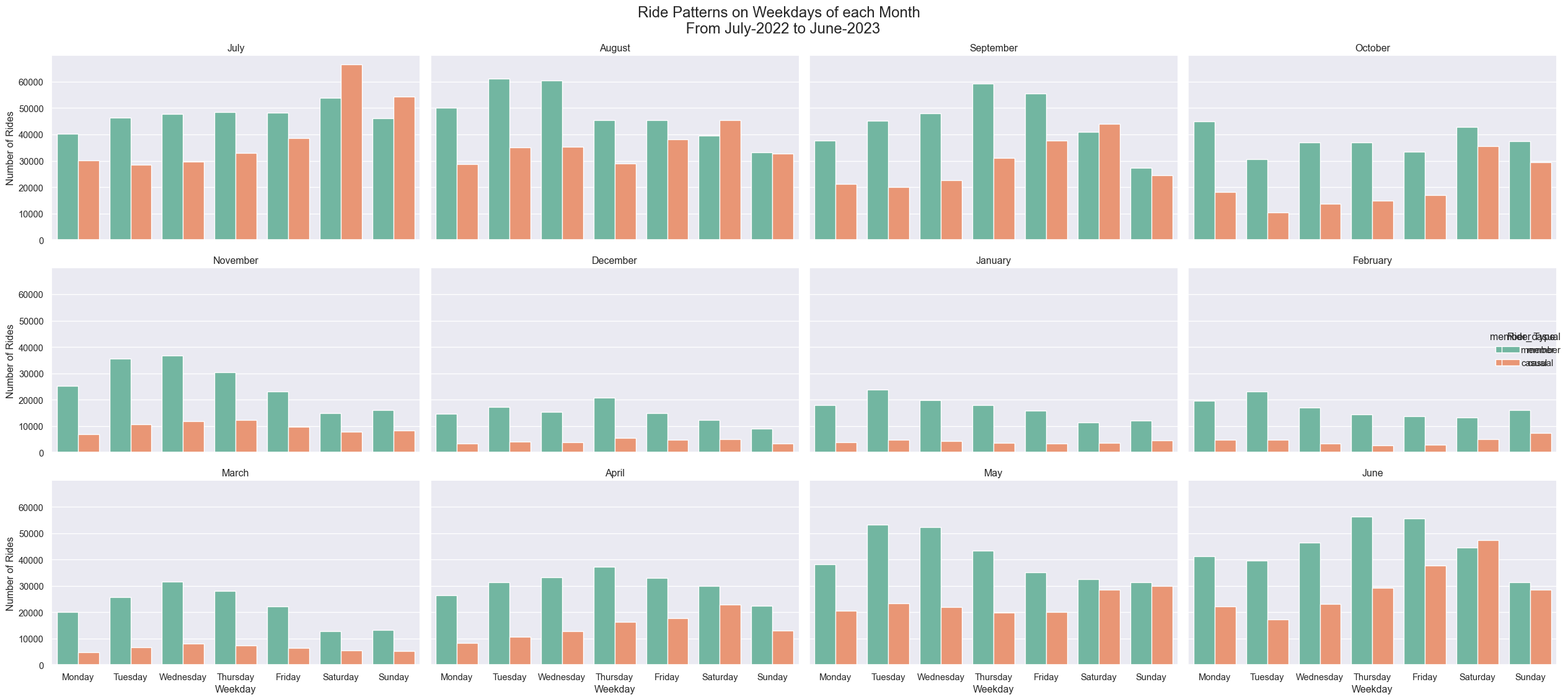
The above Figure 2 clearly shows how the number of rides change due to seasons. In winters the number of rides decrease very drastically may be because of temperature and snow. In Summers the number of rides are at its peak.
The number of rides driven by member riders increases through the week especially in working week days but for casual riders the rides increase in the weekends. The Figure 2 shows number of rides on Saturdays and Sundays by casual members overtake membership riders in the months of July and August.
Aggregating data for the visualization.
df_1year['month'] = df_1year['started_at'].dt.month_name()
df_1year['weekday'] = df_1year['started_at'].dt.day_name()

# Set categorical order for month
month_order = ['July', 'August', 'September', 'October', 'November', 'December',
             'January', 'February', 'March', 'April', 'May', 'June']
df_1year['month'] = pd.Categorical(df_1year['month'], categories=month_order, ordered=True)

# Set categorical order for weekday
weekday_order = ['Monday', 'Tuesday', 'Wednesday', 'Thursday', 'Friday', 'Saturday', 'Sunday']
df_1year['weekday'] = pd.Categorical(df_1year['weekday'], categories=weekday_order, ordered=True)


rides_on_days = df_1year.groupby(['month', 'weekday', 'member_casual']).agg(
    avg_ride_length=('ride_length', 'mean'),
    total_ride_length=('ride_length', 'sum'),
    total_rides=('ride_length', 'count')
).reset_index().sort_values(by=['month', 'weekday', 'member_casual']).round(2)

rides_on_days.head(5)| month | weekday | member_casual | avg_ride_length | total_ride_length | total_rides | |
|---|---|---|---|---|---|---|
| 0 | July | Monday | casual | 27.10 | 918148.73 | 33874 |
| 1 | July | Monday | member | 13.22 | 531467.68 | 40209 |
| 2 | July | Tuesday | casual | 22.48 | 705945.77 | 31404 |
| 3 | July | Tuesday | member | 12.69 | 588326.98 | 46353 |
| 4 | July | Wednesday | casual | 21.66 | 704094.58 | 32514 |
sns.barplot(data=rides_on_days, x='weekday', y='avg_ride_length', hue='member_casual',
            palette='Set1', errorbar=None, estimator=np.mean)
plt.title('Average Ride Length by Weekday and Rider Type')
plt.xlabel('Weekday')
plt.ylabel('Average Ride Length (minutes)')
plt.legend(title='Rider Type')
plt.xticks(rotation=45)
plt.show()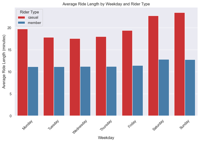
The above Figure 3 shows that the average ride length is higher for casual riders than member riders on all the days of the week. The average ride length is highest on Saturdays and Sundays for both the rider types.
sns.barplot(data=rides_on_days, x='month', y='avg_ride_length', hue='member_casual',
            palette='Set1', errorbar=None)
plt.title('Average Ride Length by Month and Rider Type')
plt.xlabel('Month')
plt.ylabel('Average Ride Length (minutes)')
plt.legend(title='Rider Type')
plt.xticks(rotation=45)
plt.show()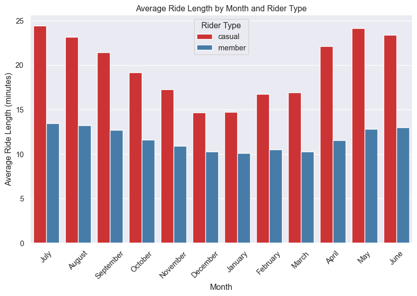
The above Figure 4 shows that the average ride length is higher for casual riders than member riders in all the months of the year. The average ride length is highest in the month of August for both the rider types.
sns.lineplot(data=rides_on_days, x='weekday', y='total_rides', hue='member_casual',
            palette='Set1', errorbar=None)
plt.title('Number of Rides by Weekday and Rider Type')
plt.xlabel('Weekday')
plt.ylabel('Number of Rides')
plt.legend(title='Rider Type')
plt.show()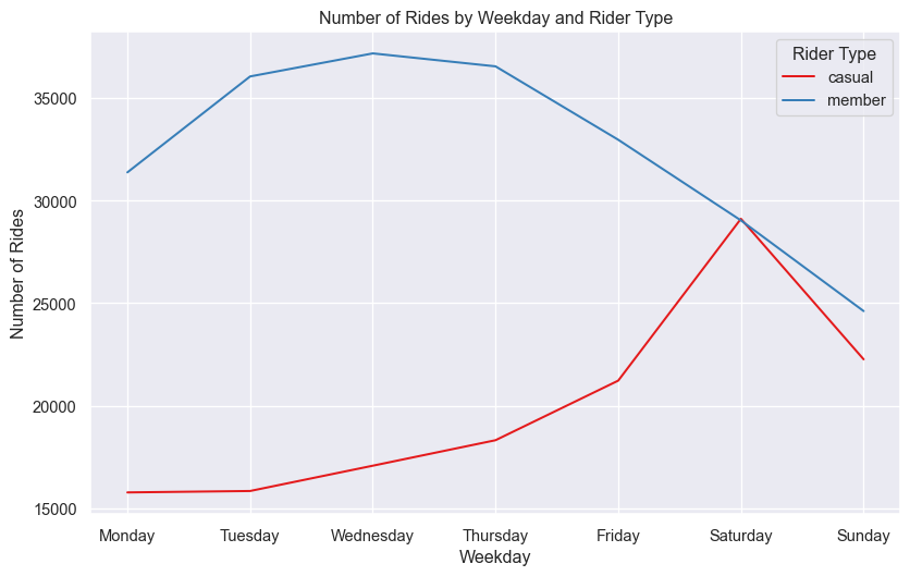
The above Figure 5 shows that the number of rides is higher for member riders than casual riders on all the days of the week. The number of rides is meet on Saturdays for both the rider types.
sns.lineplot(data=rides_on_days, x='month', y='total_rides', hue='member_casual',
            palette='Set1', errorbar=None)
plt.title('Number of Rides by Month and Rider Type')
plt.xlabel('Month')
plt.ylabel('Number of Rides')
plt.legend(title='Rider Type')
plt.show()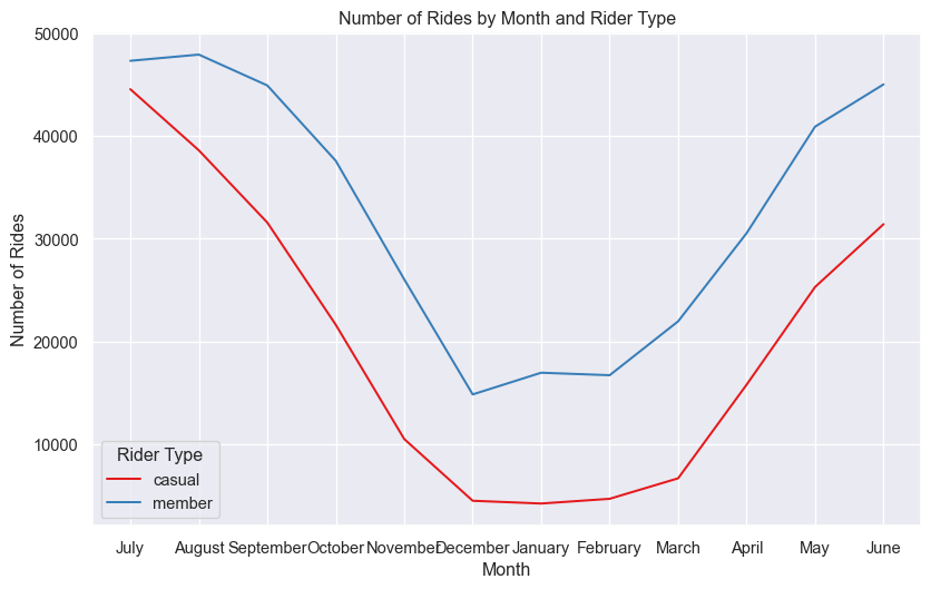
The above Figure 6 shows that the number of rides is higher for member riders than casual riders in all the months of the year. The number of rides is highest in the month of August for both the rider types.
Ride Patterns Across the Hours of the Day
- Calculating and visualizing ride patterns in a day for number of rides.
# Extracting hour from started_at
df_1year['hour'] = df_1year['started_at'].dt.hour.astype(str).str.zfill(2)  # Format hour as two digits

# Set categorical order for hour
hour_order = [f"{hour:02d}" for hour in range(24)]

df_1year['hour'] = pd.Categorical(df_1year['hour'], categories=hour_order, ordered=True)

rides_by_hour = df_1year.groupby(['hour', 'member_casual']).agg(total_rides=('ride_length', 'count')).reset_index()

sns.barplot(data=rides_by_hour, x='hour', y='total_rides', hue='member_casual',
            palette='Set1', errorbar=None)
plt.title('Ride Patterns Across the Hours of the Day')
plt.xlabel('Hour of the Day')
plt.ylabel('Number of Rides')
plt.legend(title='Rider Type')
plt.show()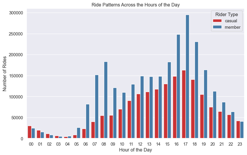
The above Figure 7 shows that the number of rides is higher for member riders than casual riders in the morning hours and evening hours. The number of rides is highest in the evening hours for both the rider types.
5 Conclusion
The analysis of the cyclist trip data reveals several key insights:
5.1 Rider Patterns
- Member riders tend to use bikes more frequently than casual riders, especially during weekdays.
- Casual riders show a preference for weekends, with a significant increase in rides during Saturdays and Sundays.
5.2 Ride Length
- The average ride length is generally longer for casual riders compared to member riders.
- The longest average ride lengths occur on weekends, particularly for casual riders.
5.3 Seasonal Trends
- The number of rides fluctuates significantly throughout the year, with peaks in summer months (July and August) and a noticeable drop in winter months (January and February).
- The analysis indicates that weather and seasonal changes have a substantial impact on cycling patterns.
- The data suggests that member riders maintain a more consistent usage pattern throughout the year compared to casual riders.
5.4 Temporal Patterns
- Ride patterns vary by time of day, with peak usage in the morning and evening hours.
- The analysis highlights the importance of understanding temporal patterns to optimize bike availability and station placements.
6 Recommendations
- Infrastructure Improvements: Consider adding more bike stations in areas with high casual rider activity, especially during weekends.
- Promotional Campaigns: Encourage casual riders to become members by offering incentives, such as discounts or free trials, to increase overall ridership.
- Seasonal Promotions: Implement seasonal promotions to boost ridership during colder months, potentially by offering discounts or special events to attract casual riders.
- Data-Driven Decisions: Continue to analyze ride patterns regularly to adapt to changing user behaviors and preferences, ensuring that the bike-sharing system remains efficient and user-friendly.