import pandas as pd
import numpy as np
import matplotlib.pyplot as plt
import seaborn as sns1 Laptop Price Prediction
This project aims to predict laptop prices based on various features such as specifications, brand, and market.
1.1 Data Description
The model is trained on the “Laptop Price Prediction Dataset” from Kaggle, which contains comprehensive laptop specifications and prices from various manufacturers.
Kaggle Dataset Link: Laptop Price Prediction Dataset
1.2 Loading Libraries and Dataset
1.2.1 Importing Libraries
Pandas, NumPy, Matplotlib, and Seaborn are used for data manipulation, numerical operations, and visualization.
Importing dataset
df = pd.read_csv("F:/Odin_school/Capstone_projects/ml_capstone/laptop.csv")

df.head()| Unnamed: 0.1 | Unnamed: 0 | Company | TypeName | Inches | ScreenResolution | Cpu | Ram | Memory | Gpu | OpSys | Weight | Price | |
|---|---|---|---|---|---|---|---|---|---|---|---|---|---|
| 0 | 0 | 0.0 | Apple | Ultrabook | 13.3 | IPS Panel Retina Display 2560x1600 | Intel Core i5 2.3GHz | 8GB | 128GB SSD | Intel Iris Plus Graphics 640 | macOS | 1.37kg | 71378.6832 |
| 1 | 1 | 1.0 | Apple | Ultrabook | 13.3 | 1440x900 | Intel Core i5 1.8GHz | 8GB | 128GB Flash Storage | Intel HD Graphics 6000 | macOS | 1.34kg | 47895.5232 |
| 2 | 2 | 2.0 | HP | Notebook | 15.6 | Full HD 1920x1080 | Intel Core i5 7200U 2.5GHz | 8GB | 256GB SSD | Intel HD Graphics 620 | No OS | 1.86kg | 30636.0000 |
| 3 | 3 | 3.0 | Apple | Ultrabook | 15.4 | IPS Panel Retina Display 2880x1800 | Intel Core i7 2.7GHz | 16GB | 512GB SSD | AMD Radeon Pro 455 | macOS | 1.83kg | 135195.3360 |
| 4 | 4 | 4.0 | Apple | Ultrabook | 13.3 | IPS Panel Retina Display 2560x1600 | Intel Core i5 3.1GHz | 8GB | 256GB SSD | Intel Iris Plus Graphics 650 | macOS | 1.37kg | 96095.8080 |
1.3 Data Cleansing
1.3.1 Checking for Missing Values
df.isnull().sum()Unnamed: 0.1 0
Unnamed: 0 30
Company 30
TypeName 30
Inches 30
ScreenResolution 30
Cpu 30
Ram 30
Memory 30
Gpu 30
OpSys 30
Weight 30
Price 30
dtype: int64All columns except Unnamed: 0.1 has missing values, which might mean that first column may just be an index column. Let’s drop it and check Unnamed: 0 column.
df = df.drop(['Unnamed: 0.1'], axis=1)

df.isnull().sum()
Unnamed: 0 30
Company 30
TypeName 30
Inches 30
ScreenResolution 30
Cpu 30
Ram 30
Memory 30
Gpu 30
OpSys 30
Weight 30
Price 30
dtype: int64Null values are still present lets drop the rows with Null values.
df = df.dropna()
df.info()
<class 'pandas.core.frame.DataFrame'>
Index: 1273 entries, 0 to 1302
Data columns (total 12 columns):
# Column Non-Null Count Dtype
--- ------ -------------- -----
0 Unnamed: 0 1273 non-null float64
1 Company 1273 non-null object
2 TypeName 1273 non-null object
3 Inches 1273 non-null object
4 ScreenResolution 1273 non-null object
5 Cpu 1273 non-null object
6 Ram 1273 non-null object
7 Memory 1273 non-null object
8 Gpu 1273 non-null object
9 OpSys 1273 non-null object
10 Weight 1273 non-null object
11 Price 1273 non-null float64
dtypes: float64(2), object(10)
memory usage: 129.3+ KBThere are 1273 non-null entries in the dataset now, which means we have successfully removed rows with missing values. Let’s check if Unnamed: 0 column is just an index column or not.
df['Unnamed: 0'].nunique()1273It seems that Unnamed: 0 column is just an index column, let’s drop it as well.
df = df.drop(['Unnamed: 0'], axis=1)
df.info()
<class 'pandas.core.frame.DataFrame'>
Index: 1273 entries, 0 to 1302
Data columns (total 11 columns):
# Column Non-Null Count Dtype
--- ------ -------------- -----
0 Company 1273 non-null object
1 TypeName 1273 non-null object
2 Inches 1273 non-null object
3 ScreenResolution 1273 non-null object
4 Cpu 1273 non-null object
5 Ram 1273 non-null object
6 Memory 1273 non-null object
7 Gpu 1273 non-null object
8 OpSys 1273 non-null object
9 Weight 1273 non-null object
10 Price 1273 non-null float64
dtypes: float64(1), object(10)
memory usage: 119.3+ KBNow we have 1273 non-null entries in the dataset and no missing values. Let’s check for duplicates in the data.
1.3.2 Checking for Duplicates
print(df.duplicated().sum())

df[df.duplicated()].sort_values(by='Company', ascending=True).head(3)29| Company | TypeName | Inches | ScreenResolution | Cpu | Ram | Memory | Gpu | OpSys | Weight | Price | |
|---|---|---|---|---|---|---|---|---|---|---|---|
| 1291 | Acer | Notebook | 15.6 | 1366x768 | Intel Celeron Dual Core N3060 1.6GHz | 4GB | 500GB HDD | Intel HD Graphics 400 | Linux | 2.4kg | 15397.92 |
| 1277 | Acer | Notebook | 15.6 | 1366x768 | Intel Celeron Dual Core N3060 1.6GHz | 4GB | 500GB HDD | Intel HD Graphics 400 | Linux | 2.4kg | 15397.92 |
| 1274 | Asus | Notebook | 15.6 | 1366x768 | Intel Celeron Dual Core N3050 1.6GHz | 4GB | 500GB HDD | Intel HD Graphics | Windows 10 | 2.2kg | 19660.32 |
There are 29 duplicate records in the dataset, let’s drop them.
df = df.drop_duplicates()

df.info()
<class 'pandas.core.frame.DataFrame'>
Index: 1244 entries, 0 to 1273
Data columns (total 11 columns):
# Column Non-Null Count Dtype
--- ------ -------------- -----
0 Company 1244 non-null object
1 TypeName 1244 non-null object
2 Inches 1244 non-null object
3 ScreenResolution 1244 non-null object
4 Cpu 1244 non-null object
5 Ram 1244 non-null object
6 Memory 1244 non-null object
7 Gpu 1244 non-null object
8 OpSys 1244 non-null object
9 Weight 1244 non-null object
10 Price 1244 non-null float64
dtypes: float64(1), object(10)
memory usage: 116.6+ KBNow we have 1244 non-null entries in the dataset and no missing values or duplicates.
There are 11 columns in the dataset, among which Price is the only column with folat64 data type rest are object data type.
1.4 Exploratory Data Analysis
Let’s start with the basic statistics of the dataset.
df.describe(include='all')| Company | TypeName | Inches | ScreenResolution | Cpu | Ram | Memory | Gpu | OpSys | Weight | Price | |
|---|---|---|---|---|---|---|---|---|---|---|---|
| count | 1244 | 1244 | 1244 | 1244 | 1244 | 1244 | 1244 | 1244 | 1244 | 1244 | 1244.000000 |
| unique | 19 | 6 | 25 | 40 | 118 | 10 | 40 | 110 | 9 | 189 | NaN |
| top | Lenovo | Notebook | 15.6 | Full HD 1920x1080 | Intel Core i5 7200U 2.5GHz | 8GB | 256GB SSD | Intel HD Graphics 620 | Windows 10 | 2.2kg | NaN |
| freq | 282 | 689 | 621 | 493 | 183 | 595 | 401 | 269 | 1022 | 106 | NaN |
| mean | NaN | NaN | NaN | NaN | NaN | NaN | NaN | NaN | NaN | NaN | 60606.224427 |
| std | NaN | NaN | NaN | NaN | NaN | NaN | NaN | NaN | NaN | NaN | 37424.636161 |
| min | NaN | NaN | NaN | NaN | NaN | NaN | NaN | NaN | NaN | NaN | 9270.720000 |
| 25% | NaN | NaN | NaN | NaN | NaN | NaN | NaN | NaN | NaN | NaN | 32655.445200 |
| 50% | NaN | NaN | NaN | NaN | NaN | NaN | NaN | NaN | NaN | NaN | 52693.920000 |
| 75% | NaN | NaN | NaN | NaN | NaN | NaN | NaN | NaN | NaN | NaN | 79813.440000 |
| max | NaN | NaN | NaN | NaN | NaN | NaN | NaN | NaN | NaN | NaN | 324954.720000 |
The dataset contains 11 columns with the following features: - Company: The brand of the laptop with 19 brands.
TypeName: The type of laptop, such as Ultrabook, Gaming, etc.
Inches: The size of the laptop screen in inches.
ScreenResolution: The resolution of the laptop screen.
Cpu: The type of CPU used in the laptop. - Ram: The amount of RAM in GB.
Memory: The type and size of storage memory (HDD/SSD).
Gpu: The type of GPU used in the laptop.
OpSys: The operating system installed on the laptop.
Weight: The weight of the laptop in kg.
Price: The price of the laptop in INR(Indian Rupees).
1.4.1 Feature Extraction
Let’s extract some features from the existing columns to make the dataset more informative.
First lets convert all the column names to lower case for consistency.
df.columns = df.columns.str.lower()

print(df.columns)
Index(['company', 'typename', 'inches', 'screenresolution', 'cpu', 'ram',
'memory', 'gpu', 'opsys', 'weight', 'price'],
dtype='object')Let’s check for the unique values in columns.
print(df.company.unique())
print(df.typename.unique())
print(df.ram.unique())
print(df.opsys.unique())
['Apple' 'HP' 'Acer' 'Asus' 'Dell' 'Lenovo' 'Chuwi' 'MSI' 'Microsoft'
'Toshiba' 'Huawei' 'Xiaomi' 'Vero' 'Razer' 'Mediacom' 'Samsung' 'Google'
'Fujitsu' 'LG']
['Ultrabook' 'Notebook' 'Gaming' '2 in 1 Convertible' 'Workstation'
'Netbook']
['8GB' '16GB' '4GB' '2GB' '12GB' '64GB' '6GB' '32GB' '24GB' '1GB']
['macOS' 'No OS' 'Windows 10' 'Mac OS X' 'Linux' 'Windows 10 S'
'Chrome OS' 'Windows 7' 'Android']print(df.cpu[1])
print(df.screenresolution[6])
print(df.gpu[88])Intel Core i5 1.8GHz
IPS Panel Retina Display 2880x1800
Nvidia GeForce GTX 1060we can seperate values in columns to form new parameters i.e,
screenresolutioncan give usdisplay_type,resolution&touchscreencpucan be seperated to formcpuandclockspeedmemorycan be seperated to formmemoryandmemory_typegpucan be seperated to getgpu_company
CPU features
# cpu brand name
df['cpu_brand'] = df.cpu.str.split().str[0]

# cpu name
df['cpu_name'] = df.cpu.str.replace(r'\d+(?:\.\d+)?GHz', '', regex=True,).str.strip()
# removing brand name
df['cpu_name'] = df.cpu_name.str.replace(r'^\w+', '', regex=True).str.strip()

# cpu clock speed
df['cpu_ghz'] = df.cpu.str.extract(r'(\d+(?:\.\d+)?)GHz').astype('float64')

df[['cpu_brand', 'cpu_name', 'cpu_ghz']]| cpu_brand | cpu_name | cpu_ghz | |
|---|---|---|---|
| 0 | Intel | Core i5 | 2.3 |
| 1 | Intel | Core i5 | 1.8 |
| 2 | Intel | Core i5 7200U | 2.5 |
| 3 | Intel | Core i7 | 2.7 |
| 4 | Intel | Core i5 | 3.1 |
| ... | ... | ... | ... |
| 1269 | Intel | Core i7 6500U | 2.5 |
| 1270 | Intel | Core i7 6500U | 2.5 |
| 1271 | Intel | Core i7 6500U | 2.5 |
| 1272 | Intel | Celeron Dual Core N3050 | 1.6 |
| 1273 | Intel | Core i7 6500U | 2.5 |
1244 rows × 3 columns
Now, we have 3 columns act as seperate features for the price prediction.
Screen Resolution Features
screenresolutionhas many features ie., screen type, screen height, width, touch screen etc. Let’s extract all of them
# display resolution
df['resolution'] = df['screenresolution'].str.extract(r'(\d+x\d+)')

# touch screen or not
df['touchscreen'] = df['screenresolution'].apply(lambda x: 1 if 'Touchscreen' in x else 0)

# Display type
df['display_type'] = df['screenresolution'].str.replace(r'\d+x\d+', "", regex = True).str.strip()

df['display_type'] = df['display_type'].str.replace(r'(Full HD|Quad HD|4K Ultra HD|/|\+|Touchscreen)', '', regex = True).str.replace('/', '', regex = True).str.strip()

df[['resolution', 'touchscreen', 'display_type']]| resolution | touchscreen | display_type | |
|---|---|---|---|
| 0 | 2560x1600 | 0 | IPS Panel Retina Display |
| 1 | 1440x900 | 0 | |
| 2 | 1920x1080 | 0 | |
| 3 | 2880x1800 | 0 | IPS Panel Retina Display |
| 4 | 2560x1600 | 0 | IPS Panel Retina Display |
| ... | ... | ... | ... |
| 1269 | 1366x768 | 0 | |
| 1270 | 1920x1080 | 1 | IPS Panel |
| 1271 | 3200x1800 | 1 | IPS Panel |
| 1272 | 1366x768 | 0 | |
| 1273 | 1366x768 | 0 |
1244 rows × 3 columns
Now, we have another 3 columns to act as 3 seperate features.
df.touchscreen.sum()np.int64(181)GPU Features
Let’s extarct gpu_brand and gpu_name from the column gpu
# gpu brand
df['gpu_brand'] = df['gpu'].str.extract(r'^(\w+)')

# gpu name
df['gpu_name'] = df['gpu'].str.replace(r'^(\w+)', '', regex = True).str.strip()

df[['gpu_brand', 'gpu_name']]| gpu_brand | gpu_name | |
|---|---|---|
| 0 | Intel | Iris Plus Graphics 640 |
| 1 | Intel | HD Graphics 6000 |
| 2 | Intel | HD Graphics 620 |
| 3 | AMD | Radeon Pro 455 |
| 4 | Intel | Iris Plus Graphics 650 |
| ... | ... | ... |
| 1269 | Nvidia | GeForce 920M |
| 1270 | Intel | HD Graphics 520 |
| 1271 | Intel | HD Graphics 520 |
| 1272 | Intel | HD Graphics |
| 1273 | AMD | Radeon R5 M330 |
1244 rows × 2 columns
Memory Features
Most of the laptops have two drives which need to be seperated and type of memory is also in the memory so we need to seperate them both after seperating the drives.
- First replace the
TBwithGB(1TB ~ 1000GB) +seperates two drives,str.split()function can be used to list the two memory drives and then they are slotted into seperate columns.
df.memory = df.memory.str.replace(r'1.0TB|1TB', "1000GB", regex = True)
df.memory = df.memory.str.replace(r'2.0TB|2TB', "2000GB", regex = True)

df.memory.unique()
array(['128GB SSD', '128GB Flash Storage', '256GB SSD', '512GB SSD',
'500GB HDD', '256GB Flash Storage', '1000GB HDD',
'128GB SSD + 1000GB HDD', '256GB SSD + 256GB SSD',
'64GB Flash Storage', '32GB Flash Storage',
'256GB SSD + 1000GB HDD', '256GB SSD + 2000GB HDD', '32GB SSD',
'2000GB HDD', '64GB SSD', '1000GB Hybrid',
'512GB SSD + 1000GB HDD', '1000GB SSD', '256GB SSD + 500GB HDD',
'128GB SSD + 2000GB HDD', '512GB SSD + 512GB SSD', '16GB SSD',
'16GB Flash Storage', '512GB SSD + 256GB SSD',
'512GB SSD + 2000GB HDD', '64GB Flash Storage + 1000GB HDD',
'180GB SSD', '1000GB HDD + 1000GB HDD', '32GB HDD',
'1000GB SSD + 1000GB HDD', '?', '512GB Flash Storage',
'128GB HDD', '240GB SSD', '8GB SSD', '508GB Hybrid',
'512GB SSD + 1000GB Hybrid', '256GB SSD + 1000GB Hybrid'],
dtype=object)df['memory_list'] = df.memory.str.split('+')
df['memory_1'] = df['memory_list'].str[0]
df['memory_2'] = df['memory_list'].str[1]
df[['memory_1', 'memory_2']]| memory_1 | memory_2 | |
|---|---|---|
| 0 | 128GB SSD | NaN |
| 1 | 128GB Flash Storage | NaN |
| 2 | 256GB SSD | NaN |
| 3 | 512GB SSD | NaN |
| 4 | 256GB SSD | NaN |
| ... | ... | ... |
| 1269 | 500GB HDD | NaN |
| 1270 | 128GB SSD | NaN |
| 1271 | 512GB SSD | NaN |
| 1272 | 64GB Flash Storage | NaN |
| 1273 | 1000GB HDD | NaN |
1244 rows × 2 columns
Let’s seperate df['memory_1'] into 2 seperate columns for memory_capacity and memory_type
df['memory_capacity_1'] = df['memory_1'].str.extract(r'(\d+)').astype('float64')
df['memory_type_1'] = df['memory_1'].str.replace(r'(\d+[A-Z]{2})', '', regex = True).str.strip()

df[['memory_capacity_1', 'memory_type_1']]| memory_capacity_1 | memory_type_1 | |
|---|---|---|
| 0 | 128.0 | SSD |
| 1 | 128.0 | Flash Storage |
| 2 | 256.0 | SSD |
| 3 | 512.0 | SSD |
| 4 | 256.0 | SSD |
| ... | ... | ... |
| 1269 | 500.0 | HDD |
| 1270 | 128.0 | SSD |
| 1271 | 512.0 | SSD |
| 1272 | 64.0 | Flash Storage |
| 1273 | 1000.0 | HDD |
1244 rows × 2 columns
Let’s repeat this for memory_2 also
df['memory_capacity_2'] = df['memory_2'].str.extract(r'(\d+)').astype('float64')
df['memory_type_2'] = df['memory_2'].str.replace(r'(\d+[A-Z]{2})', '', regex = True).str.strip()

df[['memory_capacity_2', 'memory_type_2']].dropna()| memory_capacity_2 | memory_type_2 | |
|---|---|---|
| 21 | 1000.0 | HDD |
| 28 | 256.0 | SSD |
| 37 | 1000.0 | HDD |
| 41 | 1000.0 | HDD |
| 47 | 1000.0 | HDD |
| ... | ... | ... |
| 1233 | 1000.0 | HDD |
| 1238 | 1000.0 | HDD |
| 1247 | 1000.0 | HDD |
| 1256 | 1000.0 | HDD |
| 1259 | 1000.0 | HDD |
204 rows × 2 columns
Other Features
Let’s convert all the columns that can be numeric into numeric or float i.e, ram, inches, weight
df['ram_gb'] = df['ram'].str.replace('GB', '').astype('int')

df['inches_size'] = pd.to_numeric(df['inches'], errors= 'coerce')

df['weight_kg'] = df['weight'].replace('?', np.nan).str.replace('kg', '').astype('float64')

df[['ram_gb', 'inches_size', 'weight_kg']]| ram_gb | inches_size | weight_kg | |
|---|---|---|---|
| 0 | 8 | 13.3 | 1.37 |
| 1 | 8 | 13.3 | 1.34 |
| 2 | 8 | 15.6 | 1.86 |
| 3 | 16 | 15.4 | 1.83 |
| 4 | 8 | 13.3 | 1.37 |
| ... | ... | ... | ... |
| 1269 | 4 | 15.6 | 2.20 |
| 1270 | 4 | 14.0 | 1.80 |
| 1271 | 16 | 13.3 | 1.30 |
| 1272 | 2 | 14.0 | 1.50 |
| 1273 | 6 | 15.6 | 2.19 |
1244 rows × 3 columns
Let’s look at data once more
df.info()<class 'pandas.core.frame.DataFrame'>
Index: 1244 entries, 0 to 1273
Data columns (total 29 columns):
# Column Non-Null Count Dtype
--- ------ -------------- -----
0 company 1244 non-null object
1 typename 1244 non-null object
2 inches 1244 non-null object
3 screenresolution 1244 non-null object
4 cpu 1244 non-null object
5 ram 1244 non-null object
6 memory 1244 non-null object
7 gpu 1244 non-null object
8 opsys 1244 non-null object
9 weight 1244 non-null object
10 price 1244 non-null float64
11 cpu_brand 1244 non-null object
12 cpu_name 1244 non-null object
13 cpu_ghz 1244 non-null float64
14 resolution 1244 non-null object
15 touchscreen 1244 non-null int64
16 display_type 1244 non-null object
17 gpu_brand 1244 non-null object
18 gpu_name 1244 non-null object
19 memory_list 1244 non-null object
20 memory_1 1244 non-null object
21 memory_2 204 non-null object
22 memory_capacity_1 1243 non-null float64
23 memory_type_1 1244 non-null object
24 memory_capacity_2 204 non-null float64
25 memory_type_2 204 non-null object
26 ram_gb 1244 non-null int64
27 inches_size 1243 non-null float64
28 weight_kg 1243 non-null float64
dtypes: float64(6), int64(2), object(21)
memory usage: 323.9+ KB11 columns just were made into 29 columns among which repeated columns are not necessary to build a model so let’s remove them.
df_clean = df.drop(columns = ['ram','screenresolution', 'cpu', 'memory', 'memory_list',
                              'memory_1', 'memory_2' ,'gpu', 'weight', 'inches'])

print(df_clean.info())
df_clean.head(5)
<class 'pandas.core.frame.DataFrame'>
Index: 1244 entries, 0 to 1273
Data columns (total 19 columns):
# Column Non-Null Count Dtype
--- ------ -------------- -----
0 company 1244 non-null object
1 typename 1244 non-null object
2 opsys 1244 non-null object
3 price 1244 non-null float64
4 cpu_brand 1244 non-null object
5 cpu_name 1244 non-null object
6 cpu_ghz 1244 non-null float64
7 resolution 1244 non-null object
8 touchscreen 1244 non-null int64
9 display_type 1244 non-null object
10 gpu_brand 1244 non-null object
11 gpu_name 1244 non-null object
12 memory_capacity_1 1243 non-null float64
13 memory_type_1 1244 non-null object
14 memory_capacity_2 204 non-null float64
15 memory_type_2 204 non-null object
16 ram_gb 1244 non-null int64
17 inches_size 1243 non-null float64
18 weight_kg 1243 non-null float64
dtypes: float64(6), int64(2), object(11)
memory usage: 226.7+ KB
None| company | typename | opsys | price | cpu_brand | cpu_name | cpu_ghz | resolution | touchscreen | display_type | gpu_brand | gpu_name | memory_capacity_1 | memory_type_1 | memory_capacity_2 | memory_type_2 | ram_gb | inches_size | weight_kg | |
|---|---|---|---|---|---|---|---|---|---|---|---|---|---|---|---|---|---|---|---|
| 0 | Apple | Ultrabook | macOS | 71378.6832 | Intel | Core i5 | 2.3 | 2560x1600 | 0 | IPS Panel Retina Display | Intel | Iris Plus Graphics 640 | 128.0 | SSD | NaN | NaN | 8 | 13.3 | 1.37 |
| 1 | Apple | Ultrabook | macOS | 47895.5232 | Intel | Core i5 | 1.8 | 1440x900 | 0 | Intel | HD Graphics 6000 | 128.0 | Flash Storage | NaN | NaN | 8 | 13.3 | 1.34 | |
| 2 | HP | Notebook | No OS | 30636.0000 | Intel | Core i5 7200U | 2.5 | 1920x1080 | 0 | Intel | HD Graphics 620 | 256.0 | SSD | NaN | NaN | 8 | 15.6 | 1.86 | |
| 3 | Apple | Ultrabook | macOS | 135195.3360 | Intel | Core i7 | 2.7 | 2880x1800 | 0 | IPS Panel Retina Display | AMD | Radeon Pro 455 | 512.0 | SSD | NaN | NaN | 16 | 15.4 | 1.83 |
| 4 | Apple | Ultrabook | macOS | 96095.8080 | Intel | Core i5 | 3.1 | 2560x1600 | 0 | IPS Panel Retina Display | Intel | Iris Plus Graphics 650 | 256.0 | SSD | NaN | NaN | 8 | 13.3 | 1.37 |
Now that dataset is clean let’s go for EDA.
1.4.2 Data Visualisation
As we have 8 numeric columns, let’s start with correlation plot.
sns.heatmap(df_clean.select_dtypes(include = ['int64', 'float64']).corr(),
                                   annot = True, cmap = 'coolwarm')
plt.show()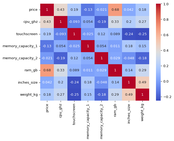
We can see that price has a strong positive correlation with ram_gb and cpu_ghz.
Let’s check the distribution of price column.
sns.histplot(df_clean['price'], bins = 20, kde = True)
plt.show()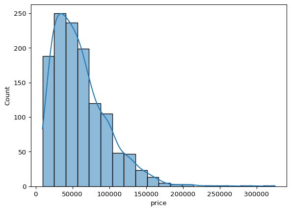
The plot is right skewed, we can log transform the price column to make it more normal.
df_clean['price_log'] = np.log1p(df_clean['price'])

sns.histplot(df_clean['price_log'], bins = 50, kde = True)
plt.show()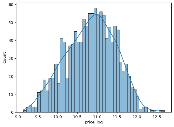
price_log is more normally distributed, let’s check the correlation of price_log with other columns.
sns.heatmap(df_clean.drop(columns = ['price']).select_dtypes(include = ['int64', 'float64']).corr(),
                                    annot = True, cmap = 'coolwarm')
plt.show()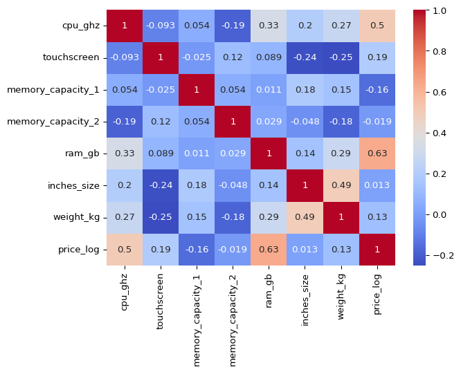
We can see that price_log has a strong positive correlation with ram_gb and cpu_ghz.
Let’s plot price_log in a boxplot to get the outliers.
ax = sns.boxplot(x='price_log', data=df_clean)
max = df_clean['price_log'].max()
plt.text(max, 0, f'{max:.2f}', ha='center', va='bottom', color='red')
plt.xlabel('Price_log')
plt.title('Boxplot of Price_log')
plt.show()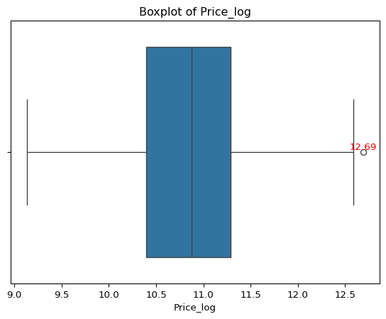
There is only one outlier in the data, let’s remove it.
df_clean = df_clean[df_clean['price_log'] < 12.6]

df_clean['price_log'].max()np.float64(12.587885975858104)Now we have removed the outliers from price_log column. Let’s look at object columns starting with companies.
sns.barplot(x = df_clean.company.value_counts().index,
            y = df_clean.company.value_counts().values)
plt.xlabel('Company')
plt.ylabel('Count')
plt.title('Company Counts')
plt.xticks(rotation = 90)
plt.show()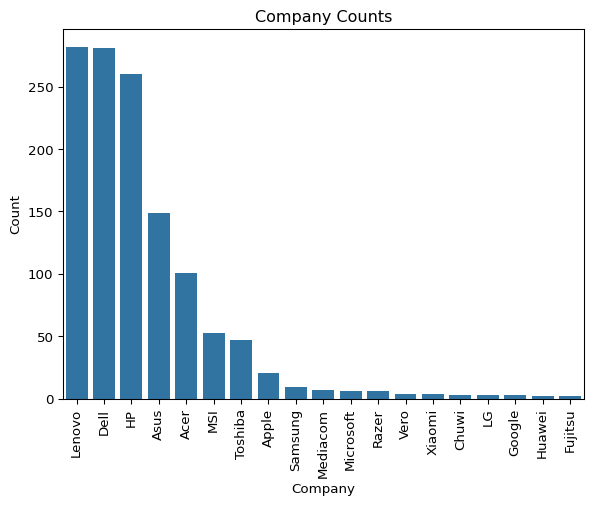
Lenovo, Dell, HP are the top 3 companies in the dataset.
company_counts = df_clean.company.value_counts()

print((company_counts[:3].sum()/len(df_clean)).round(3))0.66266.2% of the laptops are from Lenovo, Dell, HP.
Let’s look at cpu and it’s features.
print(df_clean.cpu_brand.nunique())
print(df_clean.cpu_ghz.nunique())
print(df_clean.cpu_name.nunique())
3
25
93There are 3 unique values in cpu_brand, 25 unique values in cpu_ghz, 93 unique values in cpu_name.
cpu_brand_counts = df_clean.cpu_brand.value_counts()
cpu_ghz_counts = df_clean.cpu_ghz.value_counts().sort_values(ascending = False)
cpu_name_counts = df_clean.cpu_name.value_counts()

print(cpu_brand_counts)
print(cpu_ghz_counts.head(5))
cpu_brand
Intel 1182
AMD 60
Samsung 1
Name: count, dtype: int64
cpu_ghz
2.5 278
2.8 161
2.7 158
1.6 118
2.3 84
Name: count, dtype: int64Most of the laptops have Intel CPU, 2.4GHz is the most common CPU clock speed, Intel Core i5 is the most common CPU name.
Samsung has only one laptop in the dataset, which is not ideal for building a model, let’s remove it.
df_clean = df_clean[df_clean.cpu_brand != 'Samsung']

df_clean.cpu_brand.unique()
array(['Intel', 'AMD'], dtype=object)Let’s plot cpu_ghz to know the distribution of CPU clock speed.
sns.barplot(x=cpu_ghz_counts.index.astype(str),
            y=cpu_ghz_counts.values)
plt.xlabel('CPU GHz')
plt.ylabel('Count')
plt.title('CPU GHz Distribution')
plt.xticks(rotation=90)
plt.show()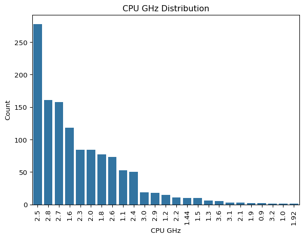
2.5GHz is the most common CPU clock speed, followed by 2.8GHz and 2.7GHz.
sns.barplot(x=df_clean.inches_size.value_counts().index.astype(str),
            y=df_clean.inches_size.value_counts().values)
plt.xlabel('Screen Size')
plt.ylabel('Count')
plt.xticks(rotation=90)
plt.title('Laptops with screen sizes')
plt.show()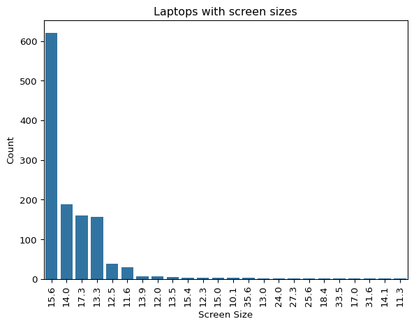
15.6 is the most common screen size, followed by 14.0 and 17.3 inches.
screen_size_counts = df_clean.inches_size.value_counts().sort_values(ascending = False)

print(screen_size_counts.head(6).sum()/screen_size_counts.sum())0.9621273166800967Only 4 sizes make up 96.21% of the laptops in the dataset, which means we can drop the other sizes.
df_clean = df_clean[df_clean.inches_size.isin([13.3, 14.0, 15.6, 17.3, 11.6, 12.5])]

df_clean.inches_size.unique()
array([13.3, 15.6, 14. , 17.3, 12.5, 11.6])Let’s look at correlation once again.
sns.heatmap(df_clean.select_dtypes(include = ['int64', 'float64']).corr(),
            annot = True, cmap = 'coolwarm')
plt.show()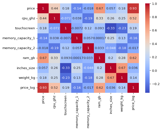
1.5 Model Building
We have gone through different parameters of the data now it’s time to put that to building a model.
I am going to build 2 models 1. Random Forest Regressor 2. Linear Regression Model
and compare them to find the best model.
1.5.1 Importing Libraries
Importing libraries for model building and evaluation with sklearn.
from sklearn.model_selection import train_test_split
from sklearn.preprocessing import LabelEncoder
from sklearn.ensemble import RandomForestRegressor
from sklearn.linear_model import LinearRegression
from sklearn.metrics import mean_squared_error, r2_score
1.5.2 Data Preparation
RandomForestRegressor can deal with Null values, so we don’t need to handle them for this model, but we need to handle them for LinearRegression model.
Let’s create a copy of the dataset and drop the price column.
Then we need to label encode the cpu_ghz, inches_size, ram_gb, memory_capacity_1, memory_capacity_2, resolution columns as they are ordinal data.
df_model = df_clean.copy().drop(columns=['price'])

ordinal_cols = ['cpu_ghz', 'inches_size', 'ram_gb', 'memory_capacity_1', 'memory_capacity_2', 'resolution', 'weight_kg']

for col in ordinal_cols:
    le = LabelEncoder()
    df_model[col] = le.fit_transform(df_model[col])

df_model.head()| company | typename | opsys | cpu_brand | cpu_name | cpu_ghz | resolution | touchscreen | display_type | gpu_brand | gpu_name | memory_capacity_1 | memory_type_1 | memory_capacity_2 | memory_type_2 | ram_gb | inches_size | weight_kg | price_log | |
|---|---|---|---|---|---|---|---|---|---|---|---|---|---|---|---|---|---|---|---|
| 0 | Apple | Ultrabook | macOS | Intel | Core i5 | 13 | 6 | 0 | IPS Panel Retina Display | Intel | Iris Plus Graphics 640 | 4 | SSD | 5 | NaN | 4 | 2 | 35 | 11.175769 |
| 1 | Apple | Ultrabook | macOS | Intel | Core i5 | 7 | 1 | 0 | Intel | HD Graphics 6000 | 4 | Flash Storage | 5 | NaN | 4 | 2 | 32 | 10.776798 | |
| 2 | HP | Notebook | No OS | Intel | Core i5 7200U | 15 | 3 | 0 | Intel | HD Graphics 620 | 7 | SSD | 5 | NaN | 4 | 4 | 69 | 10.329964 | |
| 4 | Apple | Ultrabook | macOS | Intel | Core i5 | 21 | 6 | 0 | IPS Panel Retina Display | Intel | Iris Plus Graphics 650 | 7 | SSD | 5 | NaN | 4 | 2 | 35 | 11.473111 |
| 5 | Acer | Notebook | Windows 10 | AMD | A9-Series 9420 | 20 | 0 | 0 | AMD | Radeon R5 | 8 | HDD | 5 | NaN | 2 | 4 | 90 | 9.967072 |
We need to one hot encode the cpu_brand, gpu_brand, company, display_type, touchscreen, cpu_name, gpu_name columns as they are categorical data.
nominal_cols = ['cpu_brand', 'gpu_brand', 'company', 'display_type', 'touchscreen', 'cpu_name', 'gpu_name', 'typename', 'opsys', 'memory_type_1', 'memory_type_2']

df_model = pd.get_dummies(df_model, columns=nominal_cols, drop_first=False)

print(df_model.shape)
df_model.head()
(1194, 236)| cpu_ghz | resolution | memory_capacity_1 | memory_capacity_2 | ram_gb | inches_size | weight_kg | price_log | cpu_brand_AMD | cpu_brand_Intel | ... | opsys_Windows 7 | opsys_macOS | memory_type_1_? | memory_type_1_Flash Storage | memory_type_1_HDD | memory_type_1_Hybrid | memory_type_1_SSD | memory_type_2_HDD | memory_type_2_Hybrid | memory_type_2_SSD | |
|---|---|---|---|---|---|---|---|---|---|---|---|---|---|---|---|---|---|---|---|---|---|
| 0 | 13 | 6 | 4 | 5 | 4 | 2 | 35 | 11.175769 | False | True | ... | False | True | False | False | False | False | True | False | False | False |
| 1 | 7 | 1 | 4 | 5 | 4 | 2 | 32 | 10.776798 | False | True | ... | False | True | False | True | False | False | False | False | False | False |
| 2 | 15 | 3 | 7 | 5 | 4 | 4 | 69 | 10.329964 | False | True | ... | False | False | False | False | False | False | True | False | False | False |
| 4 | 21 | 6 | 7 | 5 | 4 | 2 | 35 | 11.473111 | False | True | ... | False | True | False | False | False | False | True | False | False | False |
| 5 | 20 | 0 | 8 | 5 | 2 | 4 | 90 | 9.967072 | True | False | ... | False | False | False | False | True | False | False | False | False | False |
5 rows × 236 columns
1.5.3 Random Forest Regressor
Data Preparation
Let’s split the data into training and testing sets.
x = df_model.drop(columns = ['price_log'])
y = df_model['price_log']

x_train, x_test, y_train, y_test = train_test_split(x, y, test_size = 0.2, random_state = 42)
Model Training & Evaluation
Training the model with RandomForestRegressor and evaluating it with mean_squared_error and r2_score.
#

rf_model = RandomForestRegressor(n_estimators= 100, max_depth = 200, max_features = 20)
rf_model.fit(x_train, y_train)
RandomForestRegressor(max_depth=200, max_features=20)In a Jupyter environment, please rerun this cell to show the HTML representation or trust the notebook.
On GitHub, the HTML representation is unable to render, please try loading this page with nbviewer.org.
Parameters
| n_estimators | 100 | |
| criterion | 'squared_error' | |
| max_depth | 200 | |
| min_samples_split | 2 | |
| min_samples_leaf | 1 | |
| min_weight_fraction_leaf | 0.0 | |
| max_features | 20 | |
| max_leaf_nodes | None | |
| min_impurity_decrease | 0.0 | |
| bootstrap | True | |
| oob_score | False | |
| n_jobs | None | |
| random_state | None | |
| verbose | 0 | |
| warm_start | False | |
| ccp_alpha | 0.0 | |
| max_samples | None | |
| monotonic_cst | None |
y_pred = rf_model.predict(x_test)

mse = mean_squared_error(y_test, y_pred)
r2 = r2_score(y_test, y_pred)

print(f'Mean Squared Error: {mse:.2f}')
print(f'R2 Score: {r2:.2f}')
Mean Squared Error: 0.04
R2 Score: 0.89The R2 Score is 0.88, which is good and Mean Squared Error is 0.04 which is also good for this model.
Let’s plot the predicted vs actual values.
sns.scatterplot(x=y_test, y=y_pred)
plt.xlabel('Actual Price (log)')
plt.ylabel('Predicted Price (log)')
plt.title('Predicted vs Actual Price (log)')
plt.plot([y_test.min(), y_test.max()], [y_test.min(), y_test.max()], color='red', linestyle='--')
plt.show()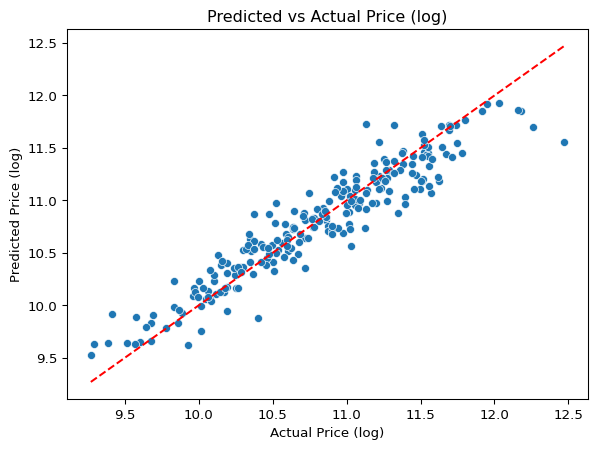
1.5.4 Linear Regression Model
Data Preparation
df_lr = df_clean.copy().drop(columns=['price'])

df_lr.info()
<class 'pandas.core.frame.DataFrame'>
Index: 1194 entries, 0 to 1273
Data columns (total 19 columns):
# Column Non-Null Count Dtype
--- ------ -------------- -----
0 company 1194 non-null object
1 typename 1194 non-null object
2 opsys 1194 non-null object
3 cpu_brand 1194 non-null object
4 cpu_name 1194 non-null object
5 cpu_ghz 1194 non-null float64
6 resolution 1194 non-null object
7 touchscreen 1194 non-null int64
8 display_type 1194 non-null object
9 gpu_brand 1194 non-null object
10 gpu_name 1194 non-null object
11 memory_capacity_1 1193 non-null float64
12 memory_type_1 1194 non-null object
13 memory_capacity_2 201 non-null float64
14 memory_type_2 201 non-null object
15 ram_gb 1194 non-null int64
16 inches_size 1194 non-null float64
17 weight_kg 1193 non-null float64
18 price_log 1194 non-null float64
dtypes: float64(6), int64(2), object(11)
memory usage: 186.6+ KBWe nedd to deal with the missing values in the dataset for LinearRegression model.
df_lr.isnull().sum()company 0
typename 0
opsys 0
cpu_brand 0
cpu_name 0
cpu_ghz 0
resolution 0
touchscreen 0
display_type 0
gpu_brand 0
gpu_name 0
memory_capacity_1 1
memory_type_1 0
memory_capacity_2 993
memory_type_2 993
ram_gb 0
inches_size 0
weight_kg 1
price_log 0
dtype: int64There are 1 missing values in weight_kg column and 1 missing value in memory_capacity_1, let’s fill it with the median and mean of the columns.
df_lr['weight_kg'] = df_lr['weight_kg'].fillna(df_lr['weight_kg'].median())
df_lr['memory_capacity_1'] = df_lr['memory_capacity_1'].fillna(df_lr['memory_capacity_1'].mean())
memory_capacity_2 and memory_type_2 are lots of missing values, let’s fill them with 0s respectively.
df_lr['memory_capacity_2'] = df_lr['memory_capacity_2'].fillna(0)
df_lr['memory_type_2'] = df_lr['memory_type_2'].fillna('None')
df_lr['memory_type_1'] = df_lr['memory_type_1'].replace({0: 'None', np.nan: 'None'})
Now we have filled the missing values in the dataset for LinearRegression model. Let’s encode the data for LinearRegression model.
ordinal_cols = ['cpu_ghz', 'inches_size', 'ram_gb', 'memory_capacity_1', 'memory_capacity_2', 'resolution', 'weight_kg']

for col in ordinal_cols:
    le = LabelEncoder()
    df_lr[col] = le.fit_transform(df_lr[col])

df_lr.head(3)| company | typename | opsys | cpu_brand | cpu_name | cpu_ghz | resolution | touchscreen | display_type | gpu_brand | gpu_name | memory_capacity_1 | memory_type_1 | memory_capacity_2 | memory_type_2 | ram_gb | inches_size | weight_kg | price_log | |
|---|---|---|---|---|---|---|---|---|---|---|---|---|---|---|---|---|---|---|---|
| 0 | Apple | Ultrabook | macOS | Intel | Core i5 | 13 | 6 | 0 | IPS Panel Retina Display | Intel | Iris Plus Graphics 640 | 4 | SSD | 0 | None | 4 | 2 | 35 | 11.175769 |
| 1 | Apple | Ultrabook | macOS | Intel | Core i5 | 7 | 1 | 0 | Intel | HD Graphics 6000 | 4 | Flash Storage | 0 | None | 4 | 2 | 32 | 10.776798 | |
| 2 | HP | Notebook | No OS | Intel | Core i5 7200U | 15 | 3 | 0 | Intel | HD Graphics 620 | 7 | SSD | 0 | None | 4 | 4 | 69 | 10.329964 |
We need to encode nominal data for LinearRegression model.
nominal_cols = ['cpu_brand', 'gpu_brand', 'company', 'display_type', 'touchscreen', 'cpu_name', 'gpu_name', 'typename', 'opsys', 'memory_type_1', 'memory_type_2']

df_lr = pd.get_dummies(df_lr, columns=nominal_cols, drop_first=False)

df_lr.head(3)| cpu_ghz | resolution | memory_capacity_1 | memory_capacity_2 | ram_gb | inches_size | weight_kg | price_log | cpu_brand_AMD | cpu_brand_Intel | ... | opsys_macOS | memory_type_1_? | memory_type_1_Flash Storage | memory_type_1_HDD | memory_type_1_Hybrid | memory_type_1_SSD | memory_type_2_HDD | memory_type_2_Hybrid | memory_type_2_None | memory_type_2_SSD | |
|---|---|---|---|---|---|---|---|---|---|---|---|---|---|---|---|---|---|---|---|---|---|
| 0 | 13 | 6 | 4 | 0 | 4 | 2 | 35 | 11.175769 | False | True | ... | True | False | False | False | False | True | False | False | True | False |
| 1 | 7 | 1 | 4 | 0 | 4 | 2 | 32 | 10.776798 | False | True | ... | True | False | True | False | False | False | False | False | True | False |
| 2 | 15 | 3 | 7 | 0 | 4 | 4 | 69 | 10.329964 | False | True | ... | False | False | False | False | False | True | False | False | True | False |
3 rows × 237 columns
Let’s split the data into training and testing sets.
x = df_lr.drop(columns = ['price_log'])
y = df_lr['price_log']

x_train, x_test, y_train, y_test = train_test_split(x, y, test_size = 0.2, random_state = 42)
Model Training & Evaluation
Training the model with LinearRegression and evaluating it with mean_squared_error and r2_score.
lr_model = LinearRegression()

lr_model.fit(x_train, y_train)LinearRegression()In a Jupyter environment, please rerun this cell to show the HTML representation or trust the notebook.
On GitHub, the HTML representation is unable to render, please try loading this page with nbviewer.org.
Parameters
| fit_intercept | True | |
| copy_X | True | |
| tol | 1e-06 | |
| n_jobs | None | |
| positive | False |
Model evaluation
y_pred = lr_model.predict(x_test)

mse = mean_squared_error(y_test, y_pred)
r2 = r2_score(y_test, y_pred)


print(f'Mean Squared Error: {mse:.2f}')
print(f'R2 Score: {r2:.2f}')
Mean Squared Error: 0.06
R2 Score: 0.85The R2 Score is 0.85, which is good and Mean Squared Error is 0.06 which is also good for this model.
Let’s plot the predicted vs actual values.
sns.scatterplot(x=y_test, y=y_pred)
plt.xlabel('Actual Price (log)')
plt.ylabel('Predicted Price (log)')
plt.title('Predicted vs Actual Price (log)')
plt.plot([y_test.min(), y_test.max()], [y_test.min(), y_test.max()], color='red', linestyle='--')
plt.show()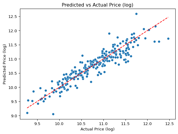
1.6 Model Featue Importance
Random Forest Regressor Features
We know that RandomForestRegressor is a tree based model, so we can use feature_importances_ to get the importance of each feature.
feature_importances = pd.DataFrame({'feature': df_model.drop(columns=['price_log']).columns, 'importance': rf_model.feature_importances_.round(4)})
feature_importances = feature_importances.sort_values('importance', ascending=False)
feature_importances.head(10)| feature | importance | |
|---|---|---|
| 4 | ram_gb | 0.1455 |
| 216 | typename_Notebook | 0.0814 |
| 1 | resolution | 0.0808 |
| 231 | memory_type_1_SSD | 0.0793 |
| 0 | cpu_ghz | 0.0749 |
| 2 | memory_capacity_1 | 0.0546 |
| 6 | weight_kg | 0.0515 |
| 229 | memory_type_1_HDD | 0.0464 |
| 5 | inches_size | 0.0278 |
| 228 | memory_type_1_Flash Storage | 0.0168 |
Linear Regression Features
We know that LinearRegression is a linear model, so we can use coef_ to get the importance of each feature.
feature_importances = pd.DataFrame({'feature': df_lr.drop(columns=['price_log']).columns, 'importance': lr_model.coef_.round(4)})
feature_importances = feature_importances.sort_values('importance', ascending=False)
feature_importances.head(10)| feature | importance | |
|---|---|---|
| 177 | gpu_name_Quadro M3000M | 0.7603 |
| 117 | gpu_name_FirePro W6150M | 0.7565 |
| 181 | gpu_name_Quadro M620M | 0.6756 |
| 91 | cpu_name_Core i7 7820HK | 0.5666 |
| 113 | cpu_name_Xeon E3-1535M v5 | 0.4989 |
| 174 | gpu_name_Quadro M2000M | 0.4989 |
| 85 | cpu_name_Core i7 6820HQ | 0.4953 |
| 149 | gpu_name_GeForce GTX1080 | 0.4902 |
| 59 | cpu_name_Core M 6Y54 | 0.4829 |
| 110 | cpu_name_Ryzen 1600 | 0.4685 |
1.6.1 Hyperparameter Tuning
I will choose RandomForestRegressor for hyperparameter tuning as it has features which are easily explainable and a tree based model can be easily tunable.
GridSearchCV is used to tune the hyperparameters of the model. n_estimators is the number of trees in the forest, max_depth is the maximum depth of the tree, max_features is the number of features to consider when looking for the best split.
from sklearn.model_selection import GridSearchCV

param_grid = {
    'n_estimators': [50, 100],
    'max_depth': [20, 30],
    'max_features': [5, 10, 15]
}

grid_search = GridSearchCV(estimator = rf_model, param_grid = param_grid, cv = 5, scoring = 'neg_mean_squared_error', verbose = 2)
grid_search.fit(x_train, y_train)print(grid_search.best_params_)
print(grid_search.best_score_){'max_depth': 30, 'max_features': 15, 'n_estimators': 100}
-0.04246258318810043grid_search.best_params_ gives the best parameters for the model depending on the scoring metric which is neg_mean_squared_error in this case.
The best parameters are n_estimators = 100, max_depth = 30, max_features = 15 and the best score is -0.042.
rf_model = RandomForestRegressor(n_estimators = 100, max_depth = 30, max_features = 15)
rf_model.fit(x_train, y_train)
RandomForestRegressor(max_depth=30, max_features=15)In a Jupyter environment, please rerun this cell to show the HTML representation or trust the notebook.
On GitHub, the HTML representation is unable to render, please try loading this page with nbviewer.org.
Parameters
| n_estimators | 100 | |
| criterion | 'squared_error' | |
| max_depth | 30 | |
| min_samples_split | 2 | |
| min_samples_leaf | 1 | |
| min_weight_fraction_leaf | 0.0 | |
| max_features | 15 | |
| max_leaf_nodes | None | |
| min_impurity_decrease | 0.0 | |
| bootstrap | True | |
| oob_score | False | |
| n_jobs | None | |
| random_state | None | |
| verbose | 0 | |
| warm_start | False | |
| ccp_alpha | 0.0 | |
| max_samples | None | |
| monotonic_cst | None |
y_pred = rf_model.predict(x_test)
mse = mean_squared_error(y_test, y_pred)
r2 = r2_score(y_test, y_pred)
print(f'Mean Squared Error: {mse:.2f}')
print(f'R2 Score: {r2:.2f}')
Mean Squared Error: 0.04
R2 Score: 0.88Even after tuning the hyper parameters, the R2 Score is 0.88 and Mean Squared Error is 0.04 which is same as the previous model, but by using this model we can save memory and time.
1.7 Conclusion
In this project, we successfully built a model to predict laptop prices based on various features. We explored the dataset, cleaned it, and extracted useful features. We built two models, RandomForestRegressor and LinearRegression, and compared their performance. The RandomForestRegressor performed better with an R2 Score of 0.88 and a Mean Squared Error of 0.04. We also tuned the hyper parameters of the model to improve its performance.
1.8 Streamlit App
The final model was deployed as a Streamlit app, which allows users to input laptop specifications and get the predicted price. The app is available at Laptop Price Prediction App.
Check out the app to see how it works and try it out with different laptop specifications.