Predict the sex of the Penguin Species

Building a model to predict the sex of three species of penguins of Palmer Penguins data.

Tip

This is my first Machine Learning project and I am still learning as of this date. This work is inspired by Julia Silge and you can find the original work by her in her blog and would like to thank her for the teachings in Julia Silge -Youtube channel

1 Exploring the data

library(tidyverse)

library(palmerpenguins)

penguins

# A tibble: 344 × 8
   species island    bill_length_mm bill_depth_mm flipper_length_mm body_mass_g
   <fct>   <fct>              <dbl>         <dbl>             <int>       <int>
 1 Adelie  Torgersen           39.1          18.7               181        3750
 2 Adelie  Torgersen           39.5          17.4               186        3800
 3 Adelie  Torgersen           40.3          18                 195        3250
 4 Adelie  Torgersen           NA            NA                  NA          NA
 5 Adelie  Torgersen           36.7          19.3               193        3450
 6 Adelie  Torgersen           39.3          20.6               190        3650
 7 Adelie  Torgersen           38.9          17.8               181        3625
 8 Adelie  Torgersen           39.2          19.6               195        4675
 9 Adelie  Torgersen           34.1          18.1               193        3475
10 Adelie  Torgersen           42            20.2               190        4250
# ℹ 334 more rows
# ℹ 2 more variables: sex <fct>, year <int>

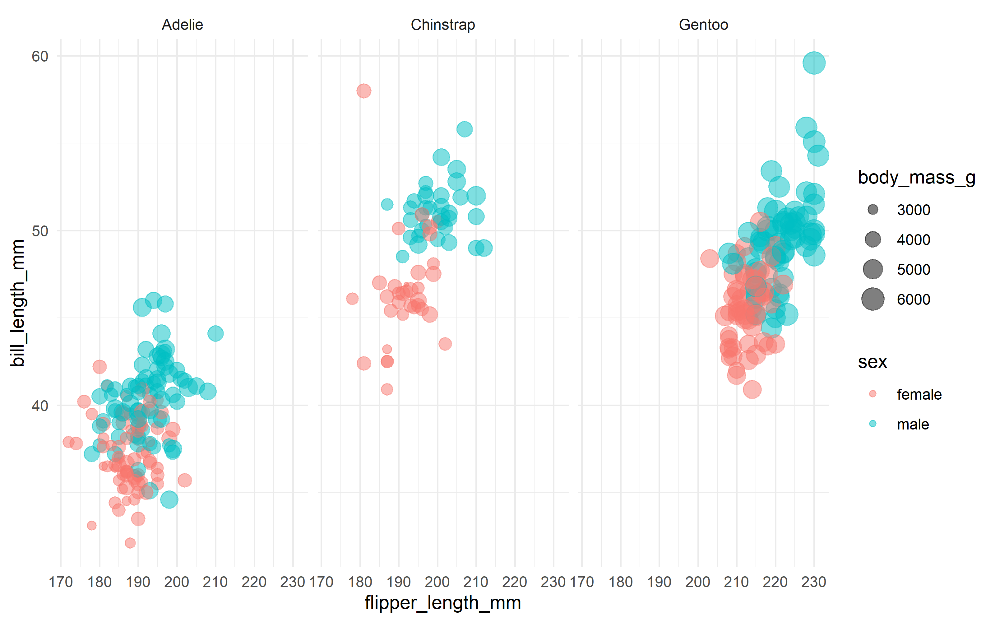
The data set is from palmerpenguins library which contains observations of Antarctic pebguins from the Palmer Archipelago. You can read more about how this dataset came to be in this post on the RStudio Education blog. Our modeling goal here is to predict the sex of the penguins using a classification model, based on other observations in the dataset.

It is easier to classify and predict species than the sex of the species as the different physical characteristics are what makes a species different from each other. But sex somewhat harder to predict.

penguins %>% filter(!is.na(sex)) %>% 
  ggplot(aes(flipper_length_mm, bill_length_mm, color = sex,
             size = body_mass_g)) +
  geom_point(alpha = 0.5) +
  facet_wrap(~species) +
  theme_minimal()

From the above graph it looks like female penguins have smaller with differet bills. Now let’s build a model but first remove year and island from the model.

penguins_df <- penguins %>% filter(!is.na(sex)) %>% select(-year, -island)

penguins_df

# A tibble: 333 × 6
   species bill_length_mm bill_depth_mm flipper_length_mm body_mass_g sex   
   <fct>            <dbl>         <dbl>             <int>       <int> <fct> 
 1 Adelie            39.1          18.7               181        3750 male  
 2 Adelie            39.5          17.4               186        3800 female
 3 Adelie            40.3          18                 195        3250 female
 4 Adelie            36.7          19.3               193        3450 female
 5 Adelie            39.3          20.6               190        3650 male  
 6 Adelie            38.9          17.8               181        3625 female
 7 Adelie            39.2          19.6               195        4675 male  
 8 Adelie            41.1          17.6               182        3200 female
 9 Adelie            38.6          21.2               191        3800 male  
10 Adelie            34.6          21.1               198        4400 male  
# ℹ 323 more rows

2 Building a Model

Let’s start by loading the tidymodels package and splitting our data into training and testing sets.

library(tidymodels)
set.seed(123)

penguin_split <- initial_split(penguins_df, strata = sex)

penguins_train <- training(penguin_split)
penguins_test <- testing(penguin_split)

As data for building a model is not that large, let’s create resamples of training data to evaluate the model.

set.seed(123)
penguin_boot <- bootstraps(penguins_train)

penguin_boot

# Bootstrap sampling 
# A tibble: 25 × 2
   splits           id         
   <list>           <chr>      
 1 <split [249/93]> Bootstrap01
 2 <split [249/91]> Bootstrap02
 3 <split [249/90]> Bootstrap03
 4 <split [249/91]> Bootstrap04
 5 <split [249/85]> Bootstrap05
 6 <split [249/87]> Bootstrap06
 7 <split [249/94]> Bootstrap07
 8 <split [249/88]> Bootstrap08
 9 <split [249/95]> Bootstrap09
10 <split [249/89]> Bootstrap10
# ℹ 15 more rows

Let’s build and compare two different models, a logistic regression model and a random forest model.

# logistic regression model
glm_spec <- logistic_reg() %>%
  set_engine("glm")

glm_spec

Logistic Regression Model Specification (classification)

Computational engine: glm 

# random forest model

rf_spec <- rand_forest() %>%
  set_mode("classification") %>% 
  set_engine("ranger")

rf_spec

Random Forest Model Specification (classification)

Computational engine: ranger 

Next let’s start putting together a tidymodels workflow(), a helper object to help manage modeling pipelines with pieces that fit together like Lego blocks. Notice that there is no model yet: Model: None.

penguin_wf <- workflow() %>% 
  add_formula(sex ~ .)

penguin_wf

══ Workflow ════════════════════════════════════════════════════════════════════
Preprocessor: Formula
Model: None

── Preprocessor ────────────────────────────────────────────────────────────────
sex ~ .

Now we can add a model and fit the model to each of the resamples. First, we can fit the logistic regression model

glm_rs <- penguin_wf %>%
  add_model(glm_spec) %>%
  fit_resamples(
    resamples = penguin_boot,
    control = control_resamples(save_pred = TRUE)
  )

→ A | warning: glm.fit: fitted probabilities numerically 0 or 1 occurred

There were issues with some computations   A: x1

There were issues with some computations   A: x3
There were issues with some computations   A: x3

glm_rs

# Resampling results
# Bootstrap sampling 
# A tibble: 25 × 5
   splits           id          .metrics         .notes           .predictions
   <list>           <chr>       <list>           <list>           <list>      
 1 <split [249/93]> Bootstrap01 <tibble [3 × 4]> <tibble [0 × 3]> <tibble>    
 2 <split [249/91]> Bootstrap02 <tibble [3 × 4]> <tibble [0 × 3]> <tibble>    
 3 <split [249/90]> Bootstrap03 <tibble [3 × 4]> <tibble [0 × 3]> <tibble>    
 4 <split [249/91]> Bootstrap04 <tibble [3 × 4]> <tibble [0 × 3]> <tibble>    
 5 <split [249/85]> Bootstrap05 <tibble [3 × 4]> <tibble [1 × 3]> <tibble>    
 6 <split [249/87]> Bootstrap06 <tibble [3 × 4]> <tibble [0 × 3]> <tibble>    
 7 <split [249/94]> Bootstrap07 <tibble [3 × 4]> <tibble [0 × 3]> <tibble>    
 8 <split [249/88]> Bootstrap08 <tibble [3 × 4]> <tibble [1 × 3]> <tibble>    
 9 <split [249/95]> Bootstrap09 <tibble [3 × 4]> <tibble [0 × 3]> <tibble>    
10 <split [249/89]> Bootstrap10 <tibble [3 × 4]> <tibble [0 × 3]> <tibble>    
# ℹ 15 more rows

There were issues with some computations:

  - Warning(s) x3: glm.fit: fitted probabilities numerically 0 or 1 occurred

Run `show_notes(.Last.tune.result)` for more information.

Second, we can fit the random forest model.

rf_rs <- penguin_wf %>%
  add_model(rf_spec) %>%
  fit_resamples(
    resamples = penguin_boot,
    control = control_resamples(save_pred = TRUE)
  )

rf_rs

# Resampling results
# Bootstrap sampling 
# A tibble: 25 × 5
   splits           id          .metrics         .notes           .predictions
   <list>           <chr>       <list>           <list>           <list>      
 1 <split [249/93]> Bootstrap01 <tibble [3 × 4]> <tibble [0 × 3]> <tibble>    
 2 <split [249/91]> Bootstrap02 <tibble [3 × 4]> <tibble [0 × 3]> <tibble>    
 3 <split [249/90]> Bootstrap03 <tibble [3 × 4]> <tibble [0 × 3]> <tibble>    
 4 <split [249/91]> Bootstrap04 <tibble [3 × 4]> <tibble [0 × 3]> <tibble>    
 5 <split [249/85]> Bootstrap05 <tibble [3 × 4]> <tibble [0 × 3]> <tibble>    
 6 <split [249/87]> Bootstrap06 <tibble [3 × 4]> <tibble [0 × 3]> <tibble>    
 7 <split [249/94]> Bootstrap07 <tibble [3 × 4]> <tibble [0 × 3]> <tibble>    
 8 <split [249/88]> Bootstrap08 <tibble [3 × 4]> <tibble [0 × 3]> <tibble>    
 9 <split [249/95]> Bootstrap09 <tibble [3 × 4]> <tibble [0 × 3]> <tibble>    
10 <split [249/89]> Bootstrap10 <tibble [3 × 4]> <tibble [0 × 3]> <tibble>    
# ℹ 15 more rows

We have fit each of our candidate models to our resampled training set!

3 Evaluate Model

Now let’s check the results and how well they performed.

collect_metrics(glm_rs)

# A tibble: 3 × 6
  .metric     .estimator   mean     n std_err .config             
  <chr>       <chr>       <dbl> <int>   <dbl> <chr>               
1 accuracy    binary     0.918     25 0.00639 Preprocessor1_Model1
2 brier_class binary     0.0585    25 0.00424 Preprocessor1_Model1
3 roc_auc     binary     0.979     25 0.00254 Preprocessor1_Model1

collect_notes(glm_rs)

# A tibble: 3 × 4
  id          location                    type    note                          
  <chr>       <chr>                       <chr>   <chr>                         
1 Bootstrap05 preprocessor 1/1, model 1/1 warning glm.fit: fitted probabilities…
2 Bootstrap08 preprocessor 1/1, model 1/1 warning glm.fit: fitted probabilities…
3 Bootstrap23 preprocessor 1/1, model 1/1 warning glm.fit: fitted probabilities…

Pretty nice! The function collect_metrics() extracts and formats the .metrics column from resampling results like the ones we have here.

collect_metrics(rf_rs)

# A tibble: 3 × 6
  .metric     .estimator   mean     n std_err .config             
  <chr>       <chr>       <dbl> <int>   <dbl> <chr>               
1 accuracy    binary     0.912     25 0.00547 Preprocessor1_Model1
2 brier_class binary     0.0664    25 0.00240 Preprocessor1_Model1
3 roc_auc     binary     0.977     25 0.00202 Preprocessor1_Model1

Let’s choose logistic regression model as it is a simpler model than random forest.

Let’s check the confusion matrix for accuracy

glm_rs %>% conf_mat_resampled()

# A tibble: 4 × 3
  Prediction Truth   Freq
  <fct>      <fct>  <dbl>
1 female     female  41.1
2 female     male     3  
3 male       female   4.4
4 male       male    42.3

Now for the roc curve which shows us how accurate a model is.

glm_rs %>%
  collect_predictions() %>%
  group_by(id) %>%
  roc_curve(sex, .pred_female) %>%
  ggplot(aes(1 - specificity, sensitivity, color = id)) +
  geom_abline(lty = 2, color = "gray80", size = 1.5) +
  geom_path(show.legend = FALSE, alpha = 0.6, linewidth = 1.2) +
  coord_equal()

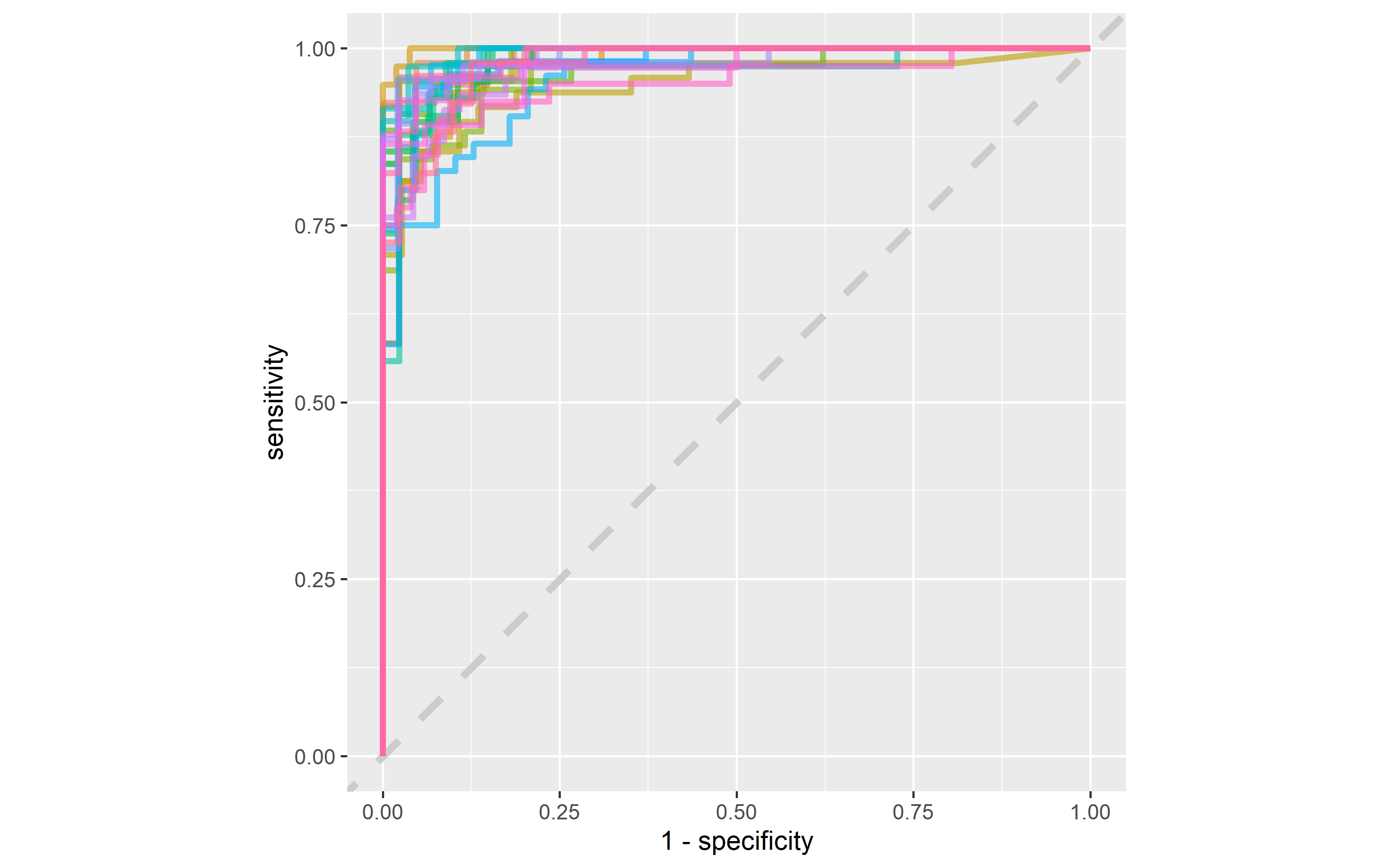
It is finally time for us to return to the testing set. Notice that we have not used the testing set yet during this whole analysis; the testing set is precious and can only be used to estimate performance on new data. Let’s fit one more time to the training data and evaluate on the testing data using the function last_fit().

penguin_final <- penguin_wf %>%
  add_model(glm_spec) %>%
  last_fit(penguin_split)

penguin_final

# Resampling results
# Manual resampling 
# A tibble: 1 × 6
  splits           id               .metrics .notes   .predictions .workflow 
  <list>           <chr>            <list>   <list>   <list>       <list>    
1 <split [249/84]> train/test split <tibble> <tibble> <tibble>     <workflow>

The metrics and predictions here are on the testing data.

collect_metrics(penguin_final)

# A tibble: 3 × 4
  .metric     .estimator .estimate .config             
  <chr>       <chr>          <dbl> <chr>               
1 accuracy    binary         0.857 Preprocessor1_Model1
2 roc_auc     binary         0.938 Preprocessor1_Model1
3 brier_class binary         0.101 Preprocessor1_Model1

collect_predictions(penguin_final) %>%
  conf_mat(sex, .pred_class)

          Truth
Prediction female male
    female     37    7
    male        5   35

penguin_final$.workflow[[1]] %>%
  tidy(exponentiate = TRUE)

# A tibble: 7 × 5
  term              estimate std.error statistic     p.value
  <chr>                <dbl>     <dbl>     <dbl>       <dbl>
1 (Intercept)       5.75e-46  19.6        -5.31  0.000000110
2 speciesChinstrap  1.37e- 4   2.34       -3.79  0.000148   
3 speciesGentoo     1.14e- 5   3.75       -3.03  0.00243    
4 bill_length_mm    1.91e+ 0   0.180       3.60  0.000321   
5 bill_depth_mm     8.36e+ 0   0.478       4.45  0.00000868 
6 flipper_length_mm 1.06e+ 0   0.0611      0.926 0.355      
7 body_mass_g       1.01e+ 0   0.00176     4.59  0.00000442 

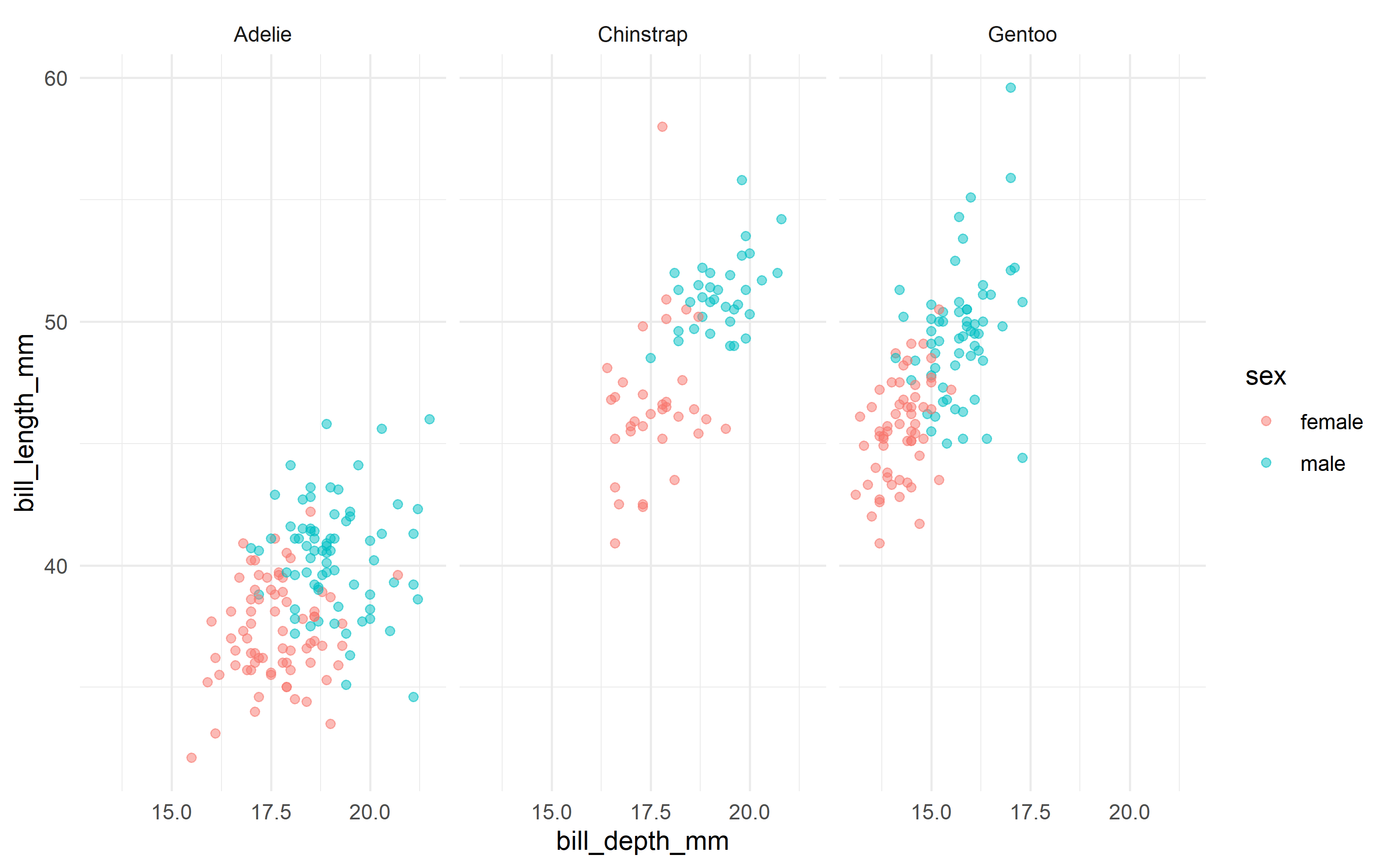
• The largest odds ratio is for bill depth, with the second largest for bill length. An increase of 1 mm in bill depth corresponds to almost 4x higher odds of being male. The characteristics of a penguin’s bill must be associated with their sex.
• We don’t have strong evidence that flipper length is different between male and female penguins, controlling for the other measures; maybe we should explore that by changing that first plot!

penguins %>% filter(!is.na(sex)) %>% 
  ggplot(aes(bill_depth_mm, bill_length_mm, color = sex)) +
  geom_point(alpha = 0.5) +
  facet_wrap(~species) +
  theme_minimal()

This graph shows much more separation between male and female penguins.