Predicting Diamonds Price
Introduction
Building a model to predict the price of the diamonds using tidymodels.
Diamonds data set is readily available to use through the ggplot2 library in the tidyverse and we will be using this data set predict the prices of the other diamonds.
In the data set various parameters of diamonds are given and each of these parameters may or may not effect the price of the diamonds.
library (tidyverse)library (plotly)library (DT)data ("diamonds" )
# A tibble: 53,940 × 10
   carat cut       color clarity depth table price     x     y     z
   <dbl> <ord>     <ord> <ord>   <dbl> <dbl> <int> <dbl> <dbl> <dbl>
 1  0.23 Ideal     E     SI2      61.5    55   326  3.95  3.98  2.43
 2  0.21 Premium   E     SI1      59.8    61   326  3.89  3.84  2.31
 3  0.23 Good      E     VS1      56.9    65   327  4.05  4.07  2.31
 4  0.29 Premium   I     VS2      62.4    58   334  4.2   4.23  2.63
 5  0.31 Good      J     SI2      63.3    58   335  4.34  4.35  2.75
 6  0.24 Very Good J     VVS2     62.8    57   336  3.94  3.96  2.48
 7  0.24 Very Good I     VVS1     62.3    57   336  3.95  3.98  2.47
 8  0.26 Very Good H     SI1      61.9    55   337  4.07  4.11  2.53
 9  0.22 Fair      E     VS2      65.1    61   337  3.87  3.78  2.49
10  0.23 Very Good H     VS1      59.4    61   338  4     4.05  2.39
# ℹ 53,930 more rows
Data has over 50,000 observations which is good for modeling.
Exploring the data
The diamonds data set is available to explore in ggplot2 library as mentioned above.
Let’s check for NA’s before exploring the data
%>% map ( ~ sum (is.na (.))) %>% unlist ()
  carat     cut   color clarity   depth   table   price       x       y       z
      0       0       0       0       0       0       0       0       0       0
It’s really good that there are no NA’s but we have to be careful of the 0 in the numeric columns.
%>% select (carat, x, y, z) %>% arrange (x, y, z)
# A tibble: 53,940 × 4
   carat     x     y     z
   <dbl> <dbl> <dbl> <dbl>
 1  1     0     0     0
 2  1.14  0     0     0
 3  1.56  0     0     0
 4  1.2   0     0     0
 5  2.25  0     0     0
 6  0.71  0     0     0
 7  0.71  0     0     0
 8  1.07  0     6.62  0
 9  0.2   3.73  3.68  2.31
10  0.2   3.73  3.71  2.33
# ℹ 53,930 more rows
Diamonds cannot have a x(length), y(width), z(depth) of 0 and have weight. So let’s replace these values with NA or we can remove them out completely too.
%>% mutate (x = if_else (x == "0" , NA , x),y = if_else (y == "0" , NA , y),z = if_else (y == "0" , NA , z)) %>% datatable ()
Now lets visualize the distribution of the diamonds.
<- diamonds %>% ggplot (aes (carat)) + geom_freqpoly (binwidth = 0.05 )ggplotly (frequency_poly)
From the Figure 1 we can observe that - Most of the diamonds are between 0.2 to 1.5 carats. - There are peaks which means higher number of diamonds at whole and common fractions.
My general knowledge is that the weight i.e, carat of the diamond influences the price most. Let’s visualize that.
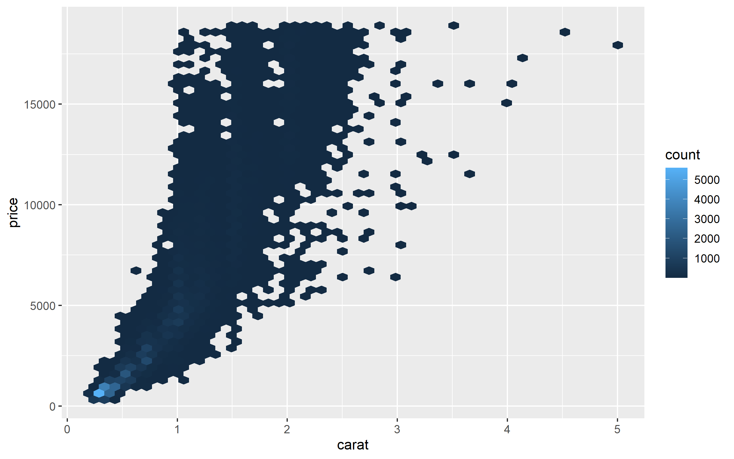
%>% ggplot (aes (carat, price)) + geom_hex (bins = 50 )
The price tends to follow exponential curve the log2() curve, we can confirm this by another graph.
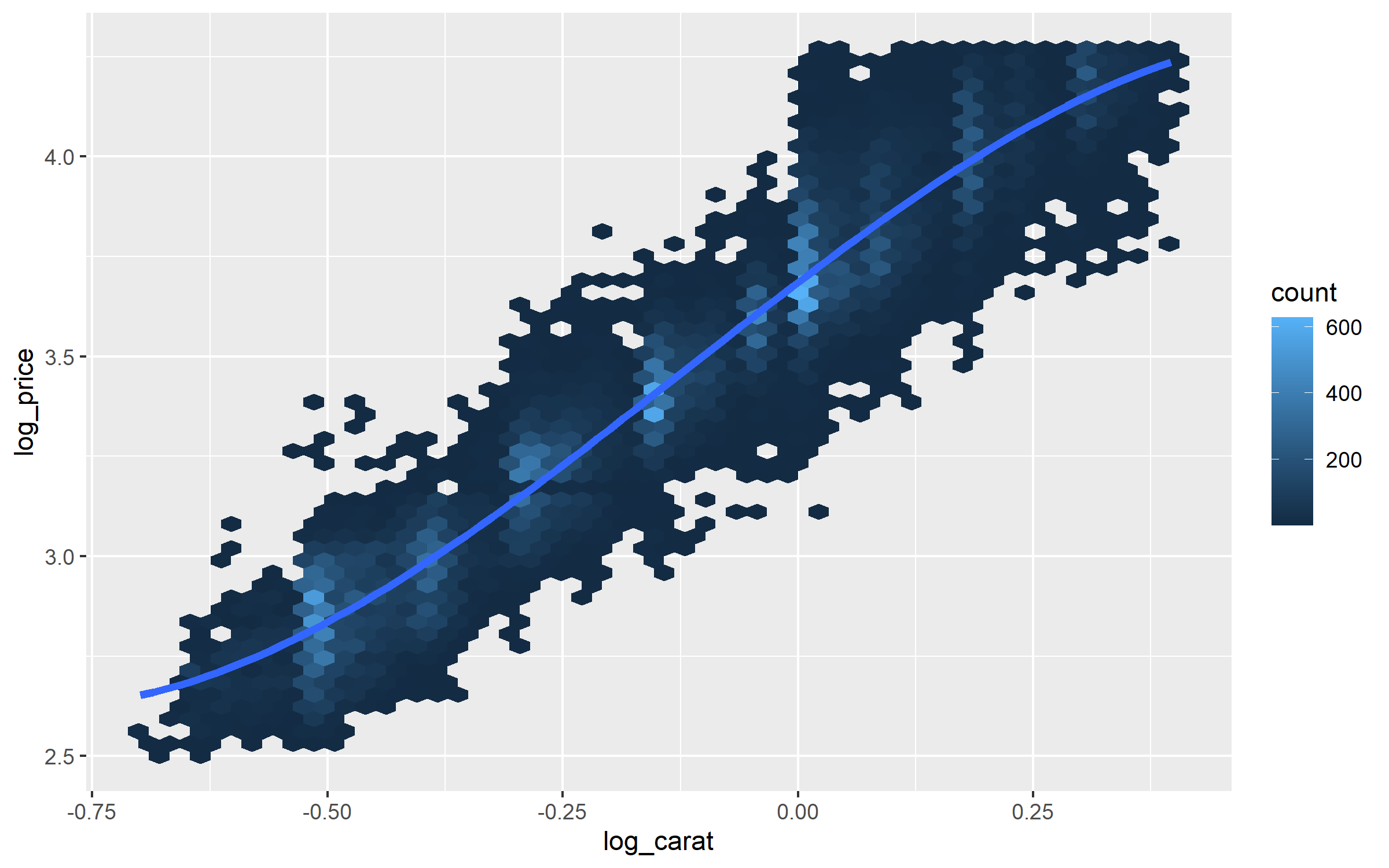
%>% filter (carat < 2.5 ) %>% mutate (log_price = log10 (price),log_carat = log10 (carat)) %>% ggplot (aes (log_carat, log_price)) + geom_hex (bins = 50 ) + geom_smooth (method = "lm" , formula = y ~ splines:: bs (x, 3 ),se = FALSE , linewidth = 1.5 )
The above Figure 2 shows that once we apply log2() to both price and carat the relationship mostly looks to be linear.
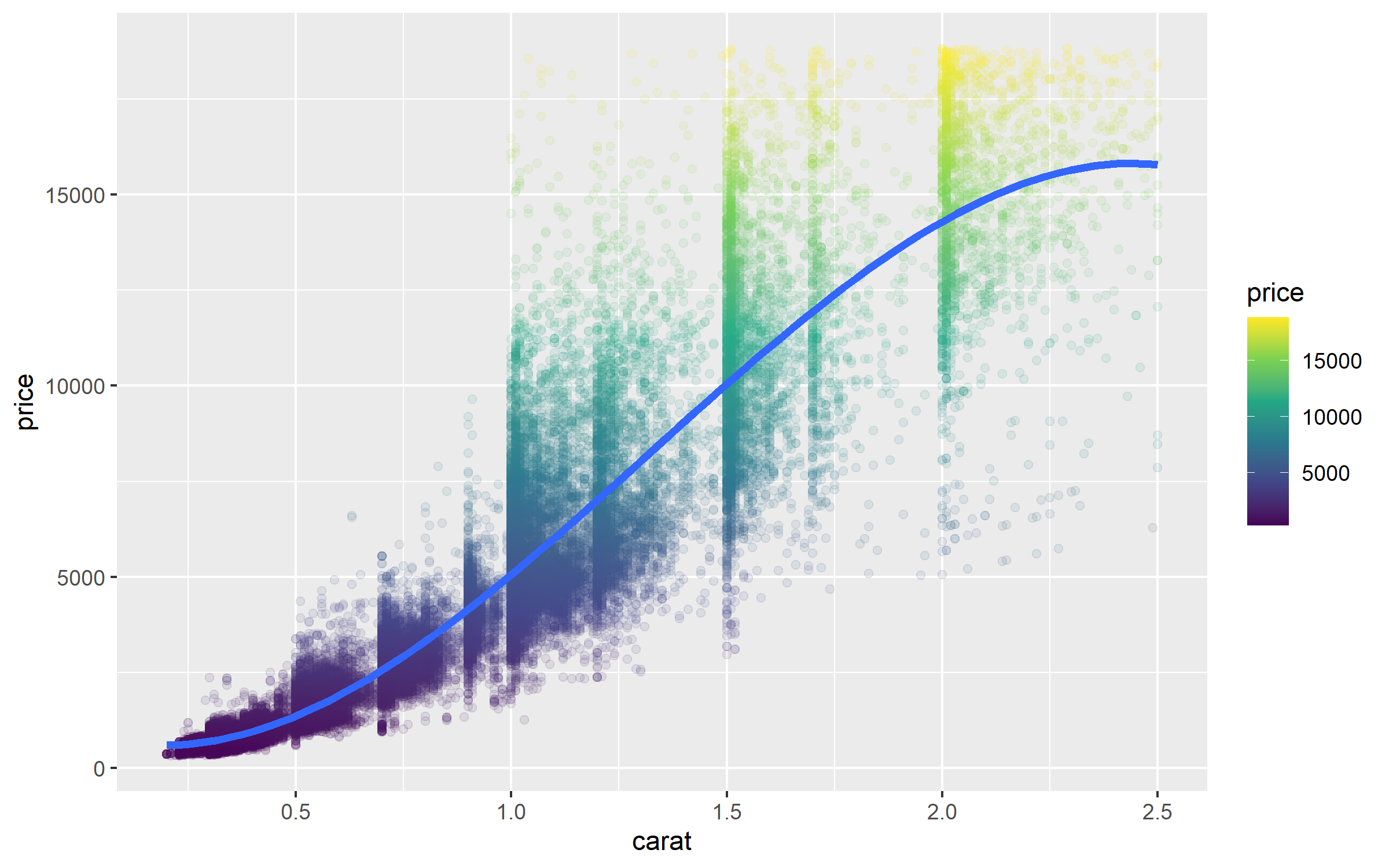
%>% filter (carat <= 2.5 ) %>% ggplot (aes (carat, price)) + geom_point (alpha = 0.1 , aes (color = price)) + geom_smooth (method = "lm" , formula = y ~ splines:: bs (x, 3 ),se = FALSE , linewidth = 1.5 ) + scale_color_viridis_c ()
We can see that price jumps when the weight is exactly or greater than to the whole and common fractions such as 0.5, 1.0, 1.5 and 2.
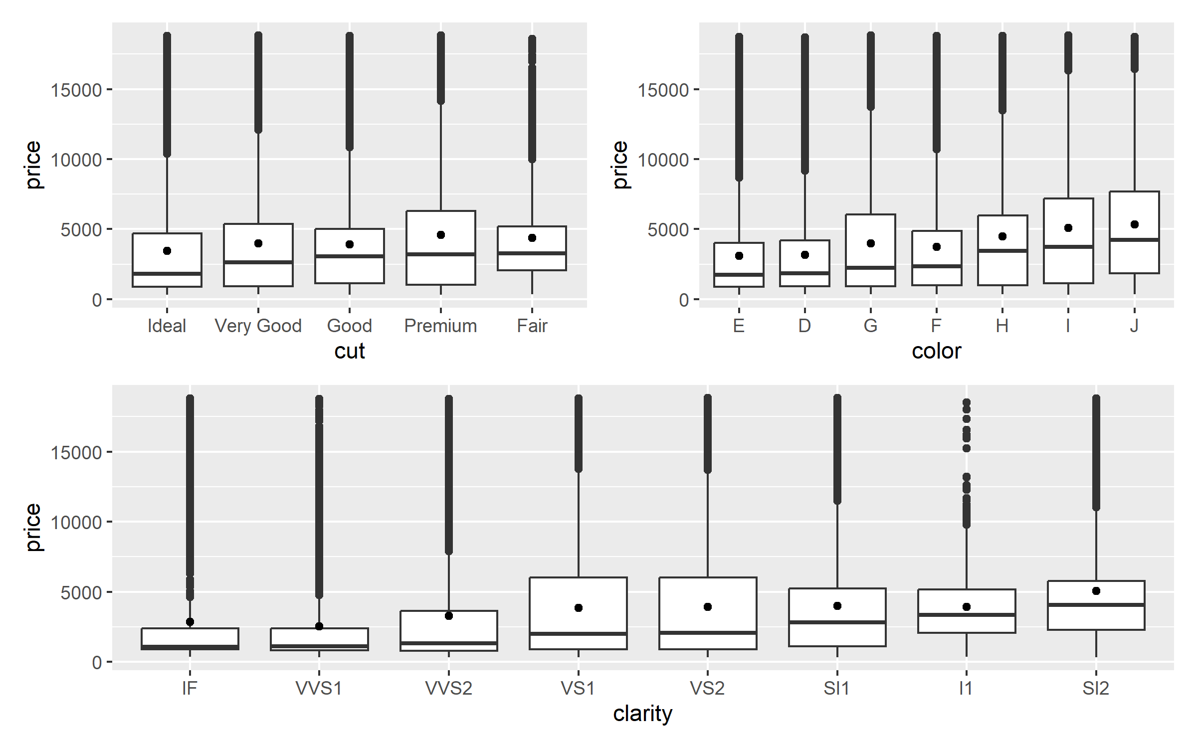
library (patchwork)<- function (param){ggplot (diamonds, aes (fct_reorder ({{param}}, price), price)) + geom_boxplot () + stat_summary (fun = mean, geom = "point" ) + labs (x = as_label (substitute (param)))plot_parameter (cut) + plot_parameter (color)) / plot_parameter (clarity))
Low quality diamonds with Fair cut and low quality color seems to have very high price. So now lets use tidymodels to model the data using rand_forest
Building a model
As every parameter in the data is important for the price prediction we are going to keep all the columns intact.
library (tidymodels)set.seed (2023 )<- diamonds %>% select (- depth) %>% mutate (price = log2 (price), carat = log2 (carat))<- initial_split (diamonds_2, strata = carat, prop = 0.8 )
<Training/Testing/Total>
<43150/10790/53940>
<- training (diamonds_split)<- testing (diamonds_split)
I am using strata with carat as most of the diamonds are not properly distributed yet all diamonds of different weight should be well represented.
<- vfold_cv (diamonds_train, strata = carat)
#  10-fold cross-validation using stratification
# A tibble: 10 × 2
   splits               id
   <list>               <chr>
 1 <split [38833/4317]> Fold01
 2 <split [38833/4317]> Fold02
 3 <split [38834/4316]> Fold03
 4 <split [38835/4315]> Fold04
 5 <split [38835/4315]> Fold05
 6 <split [38835/4315]> Fold06
 7 <split [38836/4314]> Fold07
 8 <split [38836/4314]> Fold08
 9 <split [38836/4314]> Fold09
10 <split [38837/4313]> Fold10
I think rand_forest will work better on this data set but lets compare both Linear Regression models and Random Forest models.
<- linear_reg () %>% set_engine ("glm" )
Linear Regression Model Specification (regression)

Computational engine: glm
<- rand_forest (trees = 1000 ) %>% set_mode ("regression" ) %>% set_engine ("ranger" )
Random Forest Model Specification (regression)

Main Arguments:
  trees = 1000

Computational engine: ranger
We still need to maniplulate some parts of the data like price and carat so that they are optimised which can be done using recipe library.
<- recipe (price ~ ., data = diamonds_train) %>% step_normalize (all_numeric_predictors ())<- base_recp %>% step_dummy (all_nominal_predictors ())<- ind_recp %>% step_bs (carat)
Next let’s start putting together a tidymodels workflow(), a helper object to help manage modeling pipelines with pieces that fit together like Lego blocks.
<- workflow_set (list (base_recp, ind_recp, spline_recp),list (lm_spec, rf_spec))
# A workflow set/tibble: 6 × 4
  wflow_id             info             option    result
  <chr>                <list>           <list>    <list>
1 recipe_1_linear_reg  <tibble [1 × 4]> <opts[0]> <list [0]>
2 recipe_1_rand_forest <tibble [1 × 4]> <opts[0]> <list [0]>
3 recipe_2_linear_reg  <tibble [1 × 4]> <opts[0]> <list [0]>
4 recipe_2_rand_forest <tibble [1 × 4]> <opts[0]> <list [0]>
5 recipe_3_linear_reg  <tibble [1 × 4]> <opts[0]> <list [0]>
6 recipe_3_rand_forest <tibble [1 × 4]> <opts[0]> <list [0]>
Let’s fit the two models we prepared for the data. First code block contains linear regression model and the second contains the random_forest model.
:: registerDoParallel ()<- workflow_map ("fit_resamples" ,resamples = diamonds_folds
# A workflow set/tibble: 6 × 4
  wflow_id             info             option    result
  <chr>                <list>           <list>    <list>
1 recipe_1_linear_reg  <tibble [1 × 4]> <opts[1]> <rsmp[+]>
2 recipe_1_rand_forest <tibble [1 × 4]> <opts[1]> <rsmp[+]>
3 recipe_2_linear_reg  <tibble [1 × 4]> <opts[1]> <rsmp[+]>
4 recipe_2_rand_forest <tibble [1 × 4]> <opts[1]> <rsmp[+]>
5 recipe_3_linear_reg  <tibble [1 × 4]> <opts[1]> <rsmp[+]>
6 recipe_3_rand_forest <tibble [1 × 4]> <opts[1]> <rsmp[+]>
Evaluating a model
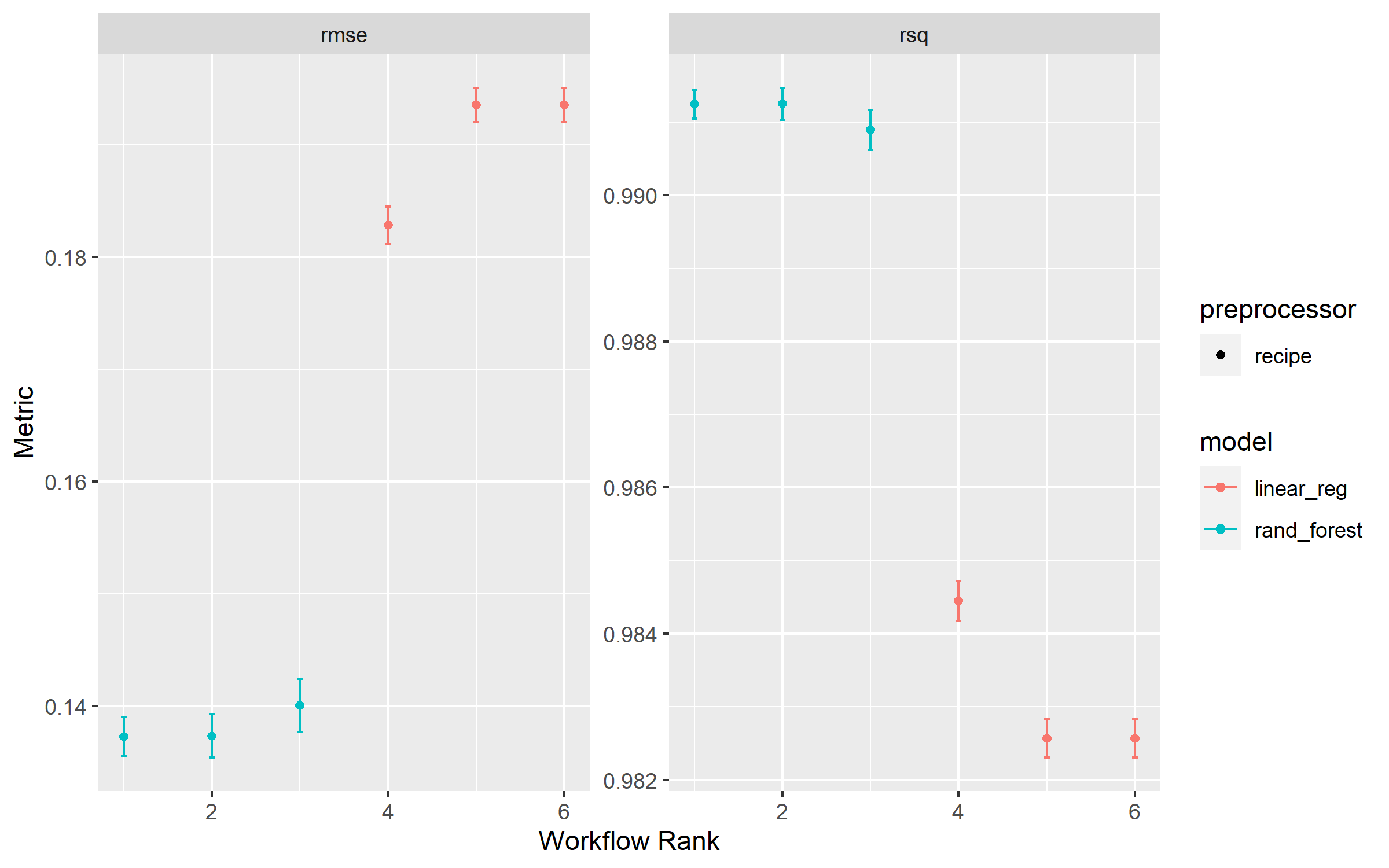
We can evaluate model by using autoplot and collect_metrics functions.
In the plot it seems that the difference between the rand_forest and linear_reg is very high but when we look at the metrics table we realise it’s not that much.
collect_metrics (diamonds_rs)
# A tibble: 12 × 9
   wflow_id         .config preproc model .metric .estimator  mean     n std_err
   <chr>            <chr>   <chr>   <chr> <chr>   <chr>      <dbl> <int>   <dbl>
 1 recipe_1_linear… Prepro… recipe  line… rmse    standard   0.194    10 9.25e-4
 2 recipe_1_linear… Prepro… recipe  line… rsq     standard   0.983    10 1.58e-4
 3 recipe_1_rand_f… Prepro… recipe  rand… rmse    standard   0.137    10 1.17e-3
 4 recipe_1_rand_f… Prepro… recipe  rand… rsq     standard   0.991    10 1.33e-4
 5 recipe_2_linear… Prepro… recipe  line… rmse    standard   0.194    10 9.25e-4
 6 recipe_2_linear… Prepro… recipe  line… rsq     standard   0.983    10 1.58e-4
 7 recipe_2_rand_f… Prepro… recipe  rand… rmse    standard   0.140    10 1.44e-3
 8 recipe_2_rand_f… Prepro… recipe  rand… rsq     standard   0.991    10 1.65e-4
 9 recipe_3_linear… Prepro… recipe  line… rmse    standard   0.183    10 1.01e-3
10 recipe_3_linear… Prepro… recipe  line… rsq     standard   0.984    10 1.67e-4
11 recipe_3_rand_f… Prepro… recipe  rand… rmse    standard   0.137    10 1.06e-3
12 recipe_3_rand_f… Prepro… recipe  rand… rsq     standard   0.991    10 1.19e-4
From the metrics table we can see that recipe_1_rand_forest seems to perform the best.
<- extract_workflow (diamonds_rs, "recipe_1_rand_forest" ) %>% fit (diamonds_train)<- pull_workflow_fit (final_fit)
parsnip model object

Ranger result

Call:
 ranger::ranger(x = maybe_data_frame(x), y = y, num.trees = ~1000,      num.threads = 1, verbose = FALSE, seed = sample.int(10^5,          1))

Type:                             Regression
Number of trees:                  1000
Sample size:                      43150
Number of independent variables:  8
Mtry:                             2
Target node size:                 5
Variable importance mode:         none
Splitrule:                        variance
OOB prediction error (MSE):       0.01859615
R squared (OOB):                  0.9913472
Let’s fit the test set to the model.
<- predict (object = final_fit,new_data = diamonds_test)
# A tibble: 10,790 × 1
   .pred
   <dbl>
 1  8.85
 2  8.64
 3  8.66
 4  8.72
 5  8.70
 6  8.62
 7  8.87
 8  8.73
 9  8.83
10  8.63
# ℹ 10,780 more rows